


PoleZeroPlot
PoleZeroPlot[expr]
gives the pole-zero plot of a rational expression expr.
PoleZeroPlot[sys]
gives the pole-zero plot of a systems model sys.
PoleZeroPlot[…,reg]
plots poles and zeros in the region reg.
更多信息

- The pole-zero plot shows the poles and zeros of a systems model sys in the complex plane.
- For a single input and single output transfer function
 , the zeros are
  and poles are
  .
. - A pole is an internal characteristic of a system and is associated with the modes and resonances that are excited by inputs such as a step input.
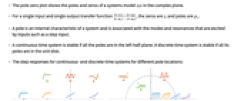
- A continuous-time system is stable if all the poles are in the left half-plane. A discrete-time system is stable if all its poles are in the unit disk.
- The step responses for continuous- and discrete-time systems for different pole locations:
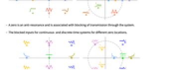
- A zero is an anti-resonance and is associated with blocking of transmission through the system.
- The blocked inputs for continuous- and discrete-time systems for different zero locations.
- The model sys can be specified as a TransferFunctionModel, StateSpaceModel, AffineStateSpaceModel, NonlinearStateSpaceModel or SystemsConnectionsModel.
- With delay systems SystemsModelDelay, there are typically infinitely many poles and zeros but only finitely many in a bounded region.
- The region specification reg can be any region in the complex plane. These include Rectangle, Disk, ImplicitRegion, etc.
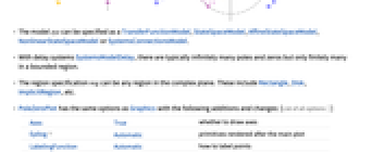
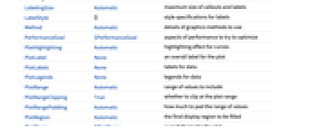
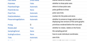
- PoleZeroPlot has the same options as Graphics with the following additions and changes: [所有选项的列表]
-
Axes True whether to draw axes Epilog Automatic primitives rendered after the main plot LabelingFunction Automatic how to label points LabelingSize Automatic maximum size of callouts and labels PerformanceGoal $PerformanceGoal aspects of performance to try to optimize PlotHighlighting Automatic highlighting effect for curves PlotLabels None labels for data PlotLegends None legends for data PlotRange Automatic range of values to include PlotRangeClipping True whether to clip at the plot range PlotTheme $PlotTheme overall theme for the plot PolarAxes False whether to draw polar axes PolarAxesOrigin Automatic where to draw polar axes PolarGridLines None polar gridlines to draw PolarTicks Automatic polar axes ticks PoleZeroMarkers Automatic markers for the poles and zeros SamplingPeriod None the sampling period ScalingFunctions None how to scale individual coordinates
所有选项的列表


范例
打开所有单元 关闭所有单元基本范例 (4)
Scope (8)
Options (15)
CoordinatesToolOptions (3)
To obtain coordinates, select the graphics and press the period key:
Obtain the coordinates in terms of the damping ratio and natural frequency:
Obtain the coordinates in terms of the damping ratio and natural frequency for a discrete-time system:
The equations to map the coordinates to the damping ratio and natural frequency:
The coordinates tool displays the coordinates in terms of the damping ratio and natural frequency:
Epilog (1)
For discrete-time systems, Epilog automatically shows a unit circle:
PolarGridLines (1)
SamplingPeriod (2)
The SamplingPeriod value determines the domain of a system given as an expression:
Applications (7)
Basic Applications (3)
Evaluate the response characteristics of a continuous-time system from the dominant pole locations:
A stable system with some overshoot:
A system with undamped oscillations:
Evaluate the response characteristics of a discrete-time system from the dominant pole locations:
A stable discrete-time system:
A stable discrete-time system with some overshoot:
A discrete-time system with undamped oscillations:
An unstable discrete-time system:
Use PoleZeroPlot along with RegionPlot to see if the poles and zeros are in specific regions:
Modal Analysis (1)
Parameter Analysis (1)
Pole-zero plots can be used to analyze the effect of a parameter on a system's transient response. Analyze the effect of the pulse ratio on the response of a DC-DC boost converter:
A PWM-switch model of the circuit:
Construct three state-space models with different pulse ratios:
The poles of the system are closer to the origin as the pulse ratio gets larger:
Increasing the pulse ratio increases the output voltage, and the oscillatory response is because the poles are on the imaginary axis:
Control Design (2)
Pole-zero plots are useful for pole-placement design. Shape the response of a mass-spring damper by interactively manipulating the pole locations:
Shape the system's response by manipulating the locations of the poles:
Pole-zero plots are useful in the LQ design to compare the poles of the open- and closed-loop systems. Compare the open- and closed-loop poles of a mixing tank:
The open-loop response to nonzero initial conditions is slow:
This is because its poles are close to the unit circle:
Design an LQ controller that improves the tank's response and obtain the closed-loop system:
The closed-loop system is faster:
This is because the closed-loop system's poles are closer to the origin:
Properties & Relations (33)
Poles (3)
The poles correspond to the modes of a system:
The pole-zero plot of the coupled two-mass spring system: »
The first pair of poles and eigenvectors generates the exponentially decaying oscillatory mode:
In this mode, the motions of the two masses are decaying, oscillatory and out of phase:
The third pole is a purely exponentially decaying mode:
To excite only this mode, the masses are given a set of equal displacements and velocities:
In this mode, the response decays exponentially:
The fourth pole that is at the origin is a purely translational mode:
To excite only this mode, both masses are given equal displacements and no velocities:
This mode is purely translational, in which the two masses move as a single unit:
The general motion of a system can be constructed from its modes:
The contribution of the modes:
The position of the first mass is the sum total of the individual modes:
So is the position of the second mass:
Poles on the stability boundary result in resonant behavior:
The sinusoid input at the resonant frequency results in a resonant response:
Zeros (5)
A system with a zero in the r.h.p at ![]() :
:
The exponential signal ![]() is blocked:
is blocked:
The zero does not cause blocking due to cancellation:
A system with a zero and a pole in the r.h.p at ![]() :
:
The exponential signal ![]() is not blocked:
is not blocked:
The response is same as that of the stable system with unstable pole and zero canceled:
A pair of complex zeros causing blocking:
Frequencies close to the zero are partially blocked, while the one matching the zero is completely blocked:
This can also be seen on the Bode plot:
For continuous-time systems, a zero with positive real part indicates an inverse response system:
For discrete-time systems, a zero outside the unit circle indicates an inverse response system:
Complex Plane Plot (2)
The open-loop poles and zeros from a RootLocusPlot:
PoleZeroPlot is a special case of RootLocusPlot:
PoleZeroPlot is a special case of ComplexListPlot:
The poles and zeros using TransferFunctionPoles and TransferFunctionZeros:
The pole-zero plot using ComplexListPlot and directly with PoleZeroPlot:
Analog Filters (5)
A Butterworth filter has no zeros and has all its poles in the left half-plane and equally spaced on the circle with radius equal to the cutoff frequency:
A Chebyshev type 1 filter has no zeros and has all its poles in the left half-plane and equally spaced on an ellipse:
A Chebyshev type 2 filter has all its zeros as conjugate pairs on the imaginary axis:
Digital Filters (11)
An IIR filter is of the form ![]() :
:
The pole count of a causal filter is greater than or equal to its zero count:
Its response to an input sequence:
The response begins with the input:
The pole count of an acausal filter is less than its zero count:
Its response to an input sequence:
The response begins before the input:
A system is stable if its region of convergence (ROC) includes the imaginary axis:
The system's impulse response:
Its ROC is to the right of the rightmost pole:
The ROC includes the left-hand side of the ![]() -plane because it is stable:
-plane because it is stable:
A system is unstable if its region of convergence (ROC) does not include the imaginary axis:
The system's impulse response:
The ROC does not include the left-hand side of the ![]() -plane because it is not stable:
-plane because it is not stable:
A discrete-time system is stable if its region of convergence (ROC) includes the unit circle:
The system's impulse response:
The ROC includes the unit circle because the system is stable:
A discrete-time system is unstable if its region of convergence (ROC) does not include the unit circle:
Its ROC does not include the unit circle because it is unstable:
A filter's phase is linear if its poles or zeros are symmetric about the unit circle:
A function to generate poles that are symmetric about the unit circle and conjugate:
A filter is invertible if all its zeros are inside the unit circle:
The inverse filter reverses the filter’s zeros and poles:
The inverse filter in series with the filter leaves the input signal unchanged:
A filter is minimum phase if it has the same number of poles and zeros and they are all inside the unit circle:
The filter and its inverse are stable, as their poles are within the unit circle:
Time Series Processes (7)
An MAProcess[{b1,…,bq},…] has q poles at the origin and q zeros:
An ARProcess[{a1,…,ap},…] has p zeros at the origin and p poles:
An ARMAProcess[{a1,…,ap},{b1,…,bq},…] has n poles and n zeros, where n=Max[p,q]:
An ARIMAProcess[{a1,…,ap},d,{b1,…,bq},…]:
Compared to an ARMAProcess, it additionally has d poles at 1 and d zeros at 0:
A SARMAProcess[{a1,…,ap},{b1,…,bq},{s,{α1,…,αm},{β1,…,βr}},…]:
It has n poles and n zeros, where n=Max[p+s m,q+s r]:
A SARIMAProcess[a,d,b,{s,{α,δ,β},…]:
Compared to a SARMAProcess, it additionally has d+δ poles at 1 and d+δ zeros at 0:
A time series is not invertible if the zeros of the transfer function lie outside the unit circle:
Check the invertibility of the process:
Since there are no zeros on the unit circle, the time series admits an invertible representation:
The zeros of the transfer function have been reflected over the unit circle:
文本
Wolfram Research (2025),PoleZeroPlot,Wolfram 语言函数,https://reference.wolfram.com/language/ref/PoleZeroPlot.html.
CMS
Wolfram 语言. 2025. "PoleZeroPlot." Wolfram 语言与系统参考资料中心. Wolfram Research. https://reference.wolfram.com/language/ref/PoleZeroPlot.html.
APA
Wolfram 语言. (2025). PoleZeroPlot. Wolfram 语言与系统参考资料中心. 追溯自 https://reference.wolfram.com/language/ref/PoleZeroPlot.html 年