Numerical Operations on Data
Numerical Operations on Data
| Mean[list] |
mean (average)
|
| Median[list] |
median (central value)
|
| Max[list] | maximum value |
| Variance[list] | variance |
| StandardDeviation[list] | standard deviation |
| Quantile[list,q] | q th quantile |
| Total[list] | total |
If the elements in list are thought of as being selected at random according to some probability distribution, then the mean gives an estimate of where the center of the distribution is located, while the standard deviation gives an estimate of how wide the dispersion in the distribution is.
The median Median[list] effectively gives the value at the halfway point in the sorted version of list. It is often considered a more robust measure of the center of a distribution than the mean, since it depends less on outlying values.
The  th quantile Quantile[list,q] effectively gives the value that is
  of the way through the sorted version of list.
For a list of length  , the Wolfram Language defines Quantile[list,q] to be s[[Ceiling[n q]]], where
  is Sort[list,Less].
There are, however, about 10 other definitions of quantile in use, all potentially giving slightly different results. The Wolfram Language covers the common cases by introducing four quantile parameters in the form Quantile[list,q,{{a,b},{c,d}}]. The parameters  and
and  in effect define where in the list should be considered a fraction
  of the way through. If this corresponds to an integer position, then the element at that position is taken to be the
  th quantile. If it is not an integer position, then a linear combination of the elements on either side is used, as specified by
  and
and  .
.
The position in a sorted list  for the
  th quantile is taken to be
  . If
. If  is an integer, then the quantile is
  . Otherwise, it is
  , with the indices taken to be
  or
or  if they are out of range.
| {{0,0},{1,0}} |
inverse empirical CDF (default)
|
| {{0,0},{0,1}} |
linear interpolation (California method)
|
| {{1/2,0},{0,0}} | element numbered closest to |
| {{1/2,0},{0,1}} |
linear interpolation (hydrologist method)
|
| {{0,1},{0,1}} | mean‐based estimate (Weibull method) |
| {{1,-1},{0,1}} | mode‐based estimate |
| {{1/3,1/3},{0,1}} | median‐based estimate |
| {{3/8,1/4},{0,1}} | normal distribution estimate |
Whenever  , the value of the
  th quantile is always equal to some actual element in list, so that the result changes discontinuously as
  varies. For
  , the
, the  th quantile interpolates linearly between successive elements in list. Median is defined to use such an interpolation.
Sometimes each item in your data may involve a list of values. The basic statistics functions in the Wolfram Language automatically apply to all corresponding elements in these lists.
Mean[{{x1, y1}, {x2, y2}, {x3, y3}}]Note that you can extract the elements in the  th "column" of a multidimensional list using list[[All,i]].
Descriptive statistics refers to properties of distributions, such as location, dispersion, and shape. The functions described here compute descriptive statistics of lists of data. You can calculate some of the standard descriptive statistics for various known distributions by using the functions described in "Continuous Distributions" and "Discrete Distributions".
The statistics are calculated assuming that each value of data  has probability equal to
  , where
  is the number of elements in the data.
| Mean[data] | average value |
| Median[data] |
median (central value)
|
| Commonest[data] | list of the elements with highest frequency |
| GeometricMean[data] | geometric mean |
| HarmonicMean[data] | harmonic mean |
| RootMeanSquare[data] | root mean square |
| TrimmedMean[data,f] | mean of remaining entries, when a fraction |
| TrimmedMean[data,{f1,f2}] | mean of remaining entries, when fractions |
| Quantile[data,q] | |
| Quartiles[data] | list of the |
Location statistics describe where the data is located. The most common functions include measures of central tendency like the mean, median, and mode. Quantile[data,q] gives the location before which  percent of the data lie. In other words, Quantile gives a value
  such that the probability that
  is less than or equal to
  and the probability that
  is greater than or equal to
  .
.
data = {6.5, 3.8, 6.6, 5.7, 6.0, 6.4, 5.3}{Mean[data], Median[data]}This is the mean when the smallest entry in the list is excluded. TrimmedMean allows you to describe the data with removed outliers:
TrimmedMean[data, {(1/7), 0}]| Variance[data] | unbiased estimate of variance, |
| StandardDeviation[data] | unbiased estimate of standard deviation |
| MeanDeviation[data] | mean absolute deviation, |
| MedianDeviation[data] | median absolute deviation, median of |
| InterquartileRange[data] | difference between the first and third quartiles |
| QuartileDeviation[data] | half the interquartile range |
Dispersion statistics summarize the scatter or spread of the data. Most of these functions describe deviation from a particular location. For instance, variance is a measure of deviation from the mean, and standard deviation is just the square root of the variance.
Variance[data]{StandardDeviation[data], MeanDeviation[data], MedianDeviation[data]}| Covariance[v1,v2] | covariance coefficient between lists v1 and v2 |
| Covariance[m] | covariance matrix for the matrix m |
| Covariance[m1,m2] | covariance matrix for the matrices m1 and m2 |
| Correlation[v1,v2] | correlation coefficient between lists v1 and v2 |
| Correlation[m] | correlation matrix for the matrix m |
| Correlation[m1,m2] | correlation matrix for the matrices m1 and m2 |
Covariance is the multivariate extension of variance. For two vectors of equal length, the covariance is a number. For a single matrix m, the i,j th element of the covariance matrix is the covariance between the i th and j th columns of m. For two matrices m1 and m2, the i,j th element of the covariance matrix is the covariance between the i th column of m1 and the j th column of m2.
While covariance measures dispersion, correlation measures association. The correlation between two vectors is equivalent to the covariance between the vectors divided by the standard deviations of the vectors. Likewise, the elements of a correlation matrix are equivalent to the elements of the corresponding covariance matrix scaled by the appropriate column standard deviations.
Covariance[data, RandomReal[1, Length[data]]]m = RandomReal[10, {20, 2}]Correlation[m]Covariance[m]Scaling the covariance matrix terms by the appropriate standard deviations gives the correlation matrix:
With[{sd = StandardDeviation[m]},
Transpose[Transpose[% / sd] / sd]]| CentralMoment[data,r] | r th central moment |
| Skewness[data] | coefficient of skewness |
| Kurtosis[data] | kurtosis coefficient |
| QuartileSkewness[data] | quartile skewness coefficient |
You can get some information about the shape of a distribution using shape statistics. Skewness describes the amount of asymmetry. Kurtosis measures the concentration of data around the peak and in the tails versus the concentration in the flanks.
Skewness is calculated by dividing the third central moment by the cube of the population standard deviation. Kurtosis is calculated by dividing the fourth central moment by the square of the population variance of the data, equivalent to CentralMoment[data,2]. (The population variance is the second central moment, and the population standard deviation is its square root.)
QuartileSkewness is calculated from the quartiles of data. It is equivalent to  , where
  ,
,  , and
, and  are the first, second, and third quartiles respectively.
CentralMoment[data, 2]A negative value for skewness indicates that the distribution underlying the data has a long left‐sided tail:
Skewness[data]| Expectation[f[x],xlist] | expected value of the function f of x with respect to the values of list |
The expectation or expected value of a function  is
is  for the list of values
  ,
,  , …,
, …,  . Many descriptive statistics are expectations. For instance, the mean is the expected value of
  , and the
  th central moment is the expected value of
  where
where  is the mean of the
  .
.
Here is the expected value of the Log of the data:
Expectation[Log[x], xdata]The functions described here are among the most commonly used discrete univariate statistical distributions. You can compute their densities, means, variances, and other related properties. The distributions themselves are represented in the symbolic form name[param1,param2,…]. Functions such as Mean, which give properties of statistical distributions, take the symbolic representation of the distribution as an argument. "Continuous Distributions" describes many continuous statistical distributions.
| BernoulliDistribution[p] | Bernoulli distribution with mean p |
| BetaBinomialDistribution[α,β,n] | binomial distribution where the success probability is a BetaDistribution[α,β] random variable |
| BetaNegativeBinomialDistribution[α,β,n] | |
negative binomial distribution where the success probability is a BetaDistribution[α,β] random variable | |
| BinomialDistribution[n,p] | binomial distribution for the number of successes that occur in n trials, where the probability of success in a trial is p |
| DiscreteUniformDistribution[{imin,imax}] | |
discrete uniform distribution over the integers from imin to imax | |
| GeometricDistribution[p] |
geometric distribution for the number of trials before the first success, where the probability of success in a trial is
p
|
| HypergeometricDistribution[n,nsucc,ntot] | |
hypergeometric distribution for the number of successes out of a sample of size n, from a population of size ntot containing nsucc successes | |
| LogSeriesDistribution[θ] | logarithmic series distribution with parameter θ |
| NegativeBinomialDistribution[n,p] | negative binomial distribution with parameters n and p |
| PoissonDistribution[μ] | Poisson distribution with mean μ |
| ZipfDistribution[ρ] | Zipf distribution with parameter ρ |
Most of the common discrete statistical distributions can be understood by considering a sequence of trials, each with two possible outcomes, for example, success and failure.
The Bernoulli distribution BernoulliDistribution[p] is the probability distribution for a single trial in which success, corresponding to value 1, occurs with probability p, and failure, corresponding to value 0, occurs with probability 1-p.
The binomial distribution BinomialDistribution[n,p] is the distribution of the number of successes that occur in n independent trials, where the probability of success in each trial is p.
The negative binomial distribution NegativeBinomialDistribution[n,p] for positive integer n is the distribution of the number of failures that occur in a sequence of trials before n successes have occurred, where the probability of success in each trial is p. The distribution is defined for any positive n, though the interpretation of n as the number of successes and p as the success probability no longer holds if n is not an integer.
The beta binomial distribution BetaBinomialDistribution[α,β,n] is a mixture of binomial and beta distributions. A BetaBinomialDistribution[α,β,n] random variable follows a BinomialDistribution[n,p] distribution, where the success probability p is itself a random variable following the beta distribution BetaDistribution[α,β]. The beta negative binomial distribution BetaNegativeBinomialDistribution[α,β,n] is a similar mixture of the beta and negative binomial distributions.
The geometric distribution GeometricDistribution[p] is the distribution of the total number of trials before the first success occurs, where the probability of success in each trial is p.
The hypergeometric distribution HypergeometricDistribution[n,nsucc,ntot] is used in place of the binomial distribution for experiments in which the n trials correspond to sampling without replacement from a population of size ntot with nsucc potential successes.
The discrete uniform distribution DiscreteUniformDistribution[{imin,imax}] represents an experiment with multiple equally probable outcomes represented by integers imin through imax.
The Poisson distribution PoissonDistribution[μ] describes the number of events that occur in a given time period where μ is the average number of events per period.
The terms in the series expansion of  about
about  are proportional to the probabilities of a discrete random variable following the logarithmic series distribution LogSeriesDistribution[θ]. The distribution of the number of items of a product purchased by a buyer in a specified interval is sometimes modeled by this distribution.
The Zipf distribution ZipfDistribution[ρ], sometimes referred to as the zeta distribution, was first used in linguistics and its use has been extended to model rare events.
| PDF[dist,x] | probability mass function at x |
| CDF[dist,x] | cumulative distribution function at x |
| InverseCDF[dist,q] | |
| Quantile[dist,q] | q th quantile |
| Mean[dist] | mean |
| Variance[dist] | variance |
| StandardDeviation[dist] | standard deviation |
| Skewness[dist] | coefficient of skewness |
| Kurtosis[dist] | coefficient of kurtosis |
| CharacteristicFunction[dist,t] | characteristic function |
| Expectation[f[x],xdist] | expectation of f[x] for x distributed according to dist |
| Median[dist] | median |
| Quartiles[dist] | list of the |
| InterquartileRange[dist] | difference between the first and third quartiles |
| QuartileDeviation[dist] | half the interquartile range |
| QuartileSkewness[dist] | quartile‐based skewness measure |
| RandomVariate[dist] | pseudorandom number with specified distribution |
| RandomVariate[dist,dims] | pseudorandom array with dimensionality dims, and elements from the specified distribution |
Distributions are represented in symbolic form. PDF[dist,x] evaluates the mass function at x if x is a numerical value, and otherwise leaves the function in symbolic form whenever possible. Similarly, CDF[dist,x] gives the cumulative distribution and Mean[dist] gives the mean of the specified distribution. The table above gives a sampling of some of the more common functions available for distributions. For a more complete description of these functions, see the description of their continuous analogues in "Continuous Distributions".
Here is a symbolic representation of the binomial distribution for 34 trials, each having probability 0.3 of success:
bdist = BinomialDistribution[34, 0.3]Mean[bdist]Mean[BinomialDistribution[n, p]]Quantile[bdist, 0.5]Expectation[x^3,x bdist]RandomVariate[bdist, {2, 3}]The functions described here are among the most commonly used continuous univariate statistical distributions. You can compute their densities, means, variances, and other related properties. The distributions themselves are represented in the symbolic form name[param1,param2,…]. Functions such as Mean, which give properties of statistical distributions, take the symbolic representation of the distribution as an argument. "Discrete Distributions" describes many common discrete univariate statistical distributions.
| NormalDistribution[μ,σ] | normal (Gaussian) distribution with mean μ and standard deviation σ |
| HalfNormalDistribution[θ] | half‐normal distribution with scale inversely proportional to parameter θ |
| LogNormalDistribution[μ,σ] | lognormal distribution based on a normal distribution with mean μ and standard deviation σ |
| InverseGaussianDistribution[μ,λ] | inverse Gaussian distribution with mean μ and scale λ |
The lognormal distribution LogNormalDistribution[μ,σ] is the distribution followed by the exponential of a normally distributed random variable. This distribution arises when many independent random variables are combined in a multiplicative fashion. The half-normal distribution HalfNormalDistribution[θ] is proportional to the distribution NormalDistribution[0,1/(θ Sqrt[2/π])] limited to the domain  .
.
The inverse Gaussian distribution InverseGaussianDistribution[μ,λ], sometimes called the Wald distribution, is the distribution of first passage times in Brownian motion with positive drift.
| ChiSquareDistribution[ν] | |
| InverseChiSquareDistribution[ν] | inverse |
| FRatioDistribution[n,m] | |
| StudentTDistribution[ν] | Student t distribution with ν degrees of freedom |
| NoncentralChiSquareDistribution[ν,λ] | noncentral |
| NoncentralStudentTDistribution[ν,δ] | noncentral Student t distribution with ν degrees of freedom and noncentrality parameter δ |
| NoncentralFRatioDistribution[n,m,λ] | noncentral |
If  , …,
, …,  are independent normal random variables with unit variance and mean zero, then
  has a
has a  distribution with
  degrees of freedom. If a normal variable is standardized by subtracting its mean and dividing by its standard deviation, then the sum of squares of such quantities follows this distribution. The
  distribution is most typically used when describing the variance of normal samples.
If  follows a
  distribution with
  degrees of freedom,
  follows the inverse
  distribution InverseChiSquareDistribution[ν]. A scaled inverse
  distribution with
  degrees of freedom and scale
  can be given as InverseChiSquareDistribution[ν,ξ]. Inverse
  distributions are commonly used as prior distributions for the variance in Bayesian analysis of normally distributed samples.
A variable that has a Student  distribution can also be written as a function of normal random variables. Let
  and
and  be independent random variables, where
  is a standard normal distribution and
  is a
is a  variable with
  degrees of freedom. In this case,
  has a
has a  distribution with
  degrees of freedom. The Student
  distribution is symmetric about the vertical axis, and characterizes the ratio of a normal variable to its standard deviation. Location and scale parameters can be included as μ and σ in StudentTDistribution[μ,σ,ν]. When
  , the
, the  distribution is the same as the Cauchy distribution.
The  ‐ratio distribution is the distribution of the ratio of two independent
  variables divided by their respective degrees of freedom. It is commonly used when comparing the variances of two populations in hypothesis testing.
Distributions that are derived from normal distributions with nonzero means are called noncentral distributions.
The sum of the squares of  normally distributed random variables with variance
  and nonzero means follows a noncentral
  distribution NoncentralChiSquareDistribution[ν,λ]. The noncentrality parameter
  is the sum of the squares of the means of the random variables in the sum. Note that in various places in the literature,
  or
or  is used as the noncentrality parameter.
The noncentral Student  distribution NoncentralStudentTDistribution[ν,δ] describes the ratio
  where
where  is a central
  random variable with
  degrees of freedom, and
  is an independent normally distributed random variable with variance
  and mean
  .
.
The noncentral  ‐ratio distribution NoncentralFRatioDistribution[n,m,λ] is the distribution of the ratio of
  to
to  , where
  is a noncentral
  random variable with noncentrality parameter
  and
and  degrees of freedom and
  is a central
  random variable with
  degrees of freedom.
| TriangularDistribution[{a,b}] | symmetric triangular distribution on the interval {a,b} |
| TriangularDistribution[{a,b},c] | triangular distribution on the interval {a,b} with maximum at c |
| UniformDistribution[{min,max}] | uniform distribution on the interval {min,max} |
The triangular distribution TriangularDistribution[{a,b},c] is a triangular distribution for  with maximum probability at
  and
and  . If
. If  is
is  , TriangularDistribution[{a,b},c] is the symmetric triangular distribution TriangularDistribution[{a,b}].
The uniform distribution UniformDistribution[{min,max}], commonly referred to as the rectangular distribution, characterizes a random variable whose value is everywhere equally likely. An example of a uniformly distributed random variable is the location of a point chosen randomly on a line from min to max.
| BetaDistribution[α,β] | continuous beta distribution with shape parameters α and β |
| CauchyDistribution[a,b] | Cauchy distribution with location parameter a and scale parameter b |
| ChiDistribution[ν] | |
| ExponentialDistribution[λ] | exponential distribution with scale inversely proportional to parameter λ |
| ExtremeValueDistribution[α,β] | extreme maximum value (Fisher–Tippett) distribution with location parameter α and scale parameter β |
| GammaDistribution[α,β] | gamma distribution with shape parameter α and scale parameter β |
| GumbelDistribution[α,β] | Gumbel minimum extreme value distribution with location parameter α and scale parameter β |
| InverseGammaDistribution[α,β] | inverse gamma distribution with shape parameter α and scale parameter β |
| LaplaceDistribution[μ,β] | Laplace (double exponential) distribution with mean μ and scale parameter β |
| LevyDistribution[μ,σ] | Lévy distribution with location parameter μ and dispersion parameter σ |
| LogisticDistribution[μ,β] | logistic distribution with mean μ and scale parameter β |
| MaxwellDistribution[σ] |
Maxwell (Maxwell
–
Boltzmann) distribution with scale parameter
σ
|
| ParetoDistribution[k,α] | Pareto distribution with minimum value parameter k and shape parameter α |
| RayleighDistribution[σ] | Rayleigh distribution with scale parameter σ |
| WeibullDistribution[α,β] | Weibull distribution with shape parameter α and scale parameter β |
If  is uniformly distributed on [-π,π], then the random variable
  follows a Cauchy distribution CauchyDistribution[a,b], with
  and
and  .
.
When  and
and  , the gamma distribution GammaDistribution[α,λ] describes the distribution of a sum of squares of
  -unit normal random variables. This form of the gamma distribution is called a
  distribution with
  degrees of freedom. When
  , the gamma distribution takes on the form of the exponential distribution ExponentialDistribution[λ], often used in describing the waiting time between events.
If a random variable  follows the gamma distribution GammaDistribution[α,β],
  follows the inverse gamma distribution InverseGammaDistribution[α,1/β]. If a random variable
  follows InverseGammaDistribution[1/2,σ/2],
  follows a Lévy distribution LevyDistribution[μ,σ].
When  and
and  have independent gamma distributions with equal scale parameters, the random variable
  follows the beta distribution BetaDistribution[α,β], where
  and
and  are the shape parameters of the gamma variables.
The  distribution ChiDistribution[ν] is followed by the square root of a
  random variable. For
  , the
, the  distribution is identical to HalfNormalDistribution[θ] with
  . For
. For  , the
, the  distribution is identical to the Rayleigh distribution RayleighDistribution[σ] with
  . For
. For  , the
, the  distribution is identical to the Maxwell–Boltzmann distribution MaxwellDistribution[σ] with
  .
.
The Laplace distribution LaplaceDistribution[μ,β] is the distribution of the difference of two independent random variables with identical exponential distributions. The logistic distribution LogisticDistribution[μ,β] is frequently used in place of the normal distribution when a distribution with longer tails is desired.
The Pareto distribution ParetoDistribution[k,α] may be used to describe income, with  representing the minimum income possible.
The Weibull distribution WeibullDistribution[α,β] is commonly used in engineering to describe the lifetime of an object. The extreme value distribution ExtremeValueDistribution[α,β] is the limiting distribution for the largest values in large samples drawn from a variety of distributions, including the normal distribution. The limiting distribution for the smallest values in such samples is the Gumbel distribution, GumbelDistribution[α,β]. The names "extreme value" and "Gumbel distribution" are sometimes used interchangeably because the distributions of the largest and smallest extreme values are related by a linear change of variable. The extreme value distribution is also sometimes referred to as the log‐Weibull distribution because of logarithmic relationships between an extreme value-distributed random variable and a properly shifted and scaled Weibull-distributed random variable.
| PDF[dist,x] | probability density function at x |
| CDF[dist,x] | cumulative distribution function at x |
| InverseCDF[dist,q] | |
| Quantile[dist,q] | q th quantile |
| Mean[dist] | mean |
| Variance[dist] | variance |
| StandardDeviation[dist] | standard deviation |
| Skewness[dist] | coefficient of skewness |
| Kurtosis[dist] | coefficient of kurtosis |
| CharacteristicFunction[dist,t] | characteristic function |
| Expectation[f[x],xdist] | expectation of f[x] for x distributed according to dist |
| Median[dist] | median |
| Quartiles[dist] | list of the |
| InterquartileRange[dist] | difference between the first and third quartiles |
| QuartileDeviation[dist] | half the interquartile range |
| QuartileSkewness[dist] | quartile‐based skewness measure |
| RandomVariate[dist] | pseudorandom number with specified distribution |
| RandomVariate[dist,dims] | pseudorandom array with dimensionality dims, and elements from the specified distribution |
The preceding table gives a list of some of the more common functions available for distributions in the Wolfram Language.
The cumulative distribution function (CDF) at  is given by the integral of the probability density function (PDF) up to
  . The PDF can therefore be obtained by differentiating the CDF (perhaps in a generalized sense). In this package the distributions are represented in symbolic form. PDF[dist,x] evaluates the density at
  if
if  is a numerical value, and otherwise leaves the function in symbolic form. Similarly, CDF[dist,x] gives the cumulative distribution.
The inverse CDF InverseCDF[dist,q] gives the value of  at which CDF[dist,x] reaches
  . The median is given by InverseCDF[dist,1/2]. Quartiles, deciles, and percentiles are particular values of the inverse CDF. Quartile skewness is equivalent to
  , where
  ,
,  , and
, and  are the first, second, and third quartiles, respectively. Inverse CDFs are used in constructing confidence intervals for statistical parameters. InverseCDF[dist,q] and Quantile[dist,q] are equivalent for continuous distributions.
The mean Mean[dist] is the expectation of the random variable distributed according to dist and is usually denoted by  . The mean is given by
  , where
  is the PDF of the distribution. The variance Variance[dist] is given by
  . The square root of the variance is called the standard deviation, and is usually denoted by
  .
.
The Skewness[dist] and Kurtosis[dist] functions give shape statistics summarizing the asymmetry and the peakedness of a distribution, respectively. Skewness is given by  and kurtosis is given by
  .
.
The characteristic function CharacteristicFunction[dist,t] is given by  . In the discrete case,
  . Each distribution has a unique characteristic function, which is sometimes used instead of the PDF to define a distribution.
The expected value Expectation[g[x],xdist] of a function g is given by  . In the discrete case, the expected value of g is given by
  .
.
RandomVariate[dist] gives pseudorandom numbers from the specified distribution.
gdist = GammaDistribution[3, 1]CDF[gdist, 10]This is the cumulative distribution function. It is given in terms of the built‐in function GammaRegularized:
cdfunction = CDF[gdist, x]Plot[cdfunction, {x, 0, 10}]RandomVariate[gdist, 5]Cluster analysis is an unsupervised learning technique used for classification of data. Data elements are partitioned into groups called clusters that represent proximate collections of data elements based on a distance or dissimilarity function. Identical element pairs have zero distance or dissimilarity, and all others have positive distance or dissimilarity.
| FindClusters[data] | partition data into lists of similar elements |
| FindClusters[data,n] | partition data into at most n lists of similar elements |
The data argument of FindClusters can be a list of data elements, associations, or rules indexing elements and labels.
| {e1,e2,…} | data specified as a list of data elements ei |
| {e1v1,e2v2,…} | data specified as a list of rules between data elements ei and labels vi |
| {e1,e2,…}{v1,v2,…} | data specified as a rule mapping data elements ei to labels vi |
| key1e1,key2e2…> | data specified as an association mapping elements ei to labels keyi |
Ways of specifying data in FindClusters.
FindClusters works for a variety of data types, including numerical, textual, and image, as well as Boolean vectors, dates and times. All data elements ei must have the same dimensions.
data = {1.2, 9.1, 2.3, 35.4, 35.7, 71.8};FindClusters clusters the numbers based on their proximity:
FindClusters[data]The rule-based data syntax allows for clustering data elements and returning labels for those elements.
data1 = {{1, 2}, {5, 7}, {0, 2}, {4, 7}} ;
FindClusters[data1 -> Range[Length[data1]]]
The rule-based data syntax can also be used to cluster data based on parts of each data entry. For instance, you might want to cluster data in a data table while ignoring particular columns in the table.
datarecords = {{"Joe", "Smith", 158, 64.4}, {"Mary", "Davis", 137, 64.4}, {"Bob", "Lewis", 141, 62.8}, {"John", "Thompson", 235, 71.1}, {"Lewis", "Black", 225, 71.4}, {"Sally", "Jones", 168, 62.}, {"Tom", "Smith", 243, 70.9}, {"Jane", "Doe", 225, 71.4}};FindClusters[Drop[datarecords, None, {1, 2}] -> datarecords]In principle, it is possible to cluster points given in an arbitrary number of dimensions. However, it is difficult at best to visualize the clusters above two or three dimensions. To compare optional methods in this documentation, an easily visualizable set of two-dimensional data will be used.
The following commands define a set of 300 two-dimensional data points chosen to group into four somewhat nebulous clusters:
GaussianRandomData[n_Integer, p_, sigma_] := Table[p + {Re[#], Im[#]}&[RandomReal[NormalDistribution[0, sigma]]E^I RandomReal[{0, 2π}]], {n}];
datapairs = BlockRandom[
	SeedRandom[1234];
	Join[GaussianRandomData[100, {2, 1}, .3], GaussianRandomData[100, {1, 1.8}, .2],
GaussianRandomData[100, {1, 1.1}, .4], GaussianRandomData[100, {1.75, 1.75}, 0.1]]];cl = FindClusters[datapairs];ListPlot[cl]With the default settings, FindClusters has found the four clusters of points.
You can also direct FindClusters to find a specific number of clusters.
ListPlot[FindClusters[datapairs, 3]]ListPlot[FindClusters[datapairs, 5]]option name | default value | |
| CriterionFunction | Automatic | criterion for selecting a method |
| DistanceFunction | Automatic | the distance function to use |
| Method | Automatic | the clustering method to use |
| PerformanceGoal | Automatic | aspect of performance to optimize |
| Weights | Automatic | what weight to give to each example |
Options for FindClusters.
In principle, clustering techniques can be applied to any set of data. All that is needed is a measure of how far apart each element in the set is from other elements, that is, a function giving the distance between elements.
FindClusters[{e1,e2,…},DistanceFunction->f] treats pairs of elements as being less similar when their distances f[ei,ej] are larger. The function f can be any appropriate distance or dissimilarity function. A dissimilarity function f satisfies the following:

If the ei are vectors of numbers, FindClusters by default uses a squared Euclidean distance. If the ei are lists of Boolean True and False (or 0 and 1) elements, FindClusters by default uses a dissimilarity based on the normalized fraction of elements that disagree. If the ei are strings, FindClusters by default uses a distance function based on the number of point changes needed to get from one string to another.
| EuclideanDistance[u,v] | the Euclidean norm |
| SquaredEuclideanDistance[u,v] | squared Euclidean norm |
| ManhattanDistance[u,v] | the Manhattan distance |
| ChessboardDistance[u,v] | the chessboard or Chebyshev distance |
| CanberraDistance[u,v] | the Canberra distance |
| CosineDistance[u,v] | the cosine distance |
| CorrelationDistance[u,v] | |
| BrayCurtisDistance[u,v] | the Bray–Curtis distance |
ListPlot[FindClusters[datapairs, DistanceFunction -> ManhattanDistance]]Dissimilarities for Boolean vectors are typically calculated by comparing the elements of two Boolean vectors  and
and  pairwise. It is convenient to summarize each dissimilarity function in terms of
  , where
  is the number of corresponding pairs of elements in
  and
and  , respectively, equal to
  and
and  . The number
  counts the pairs
  in
in  , with
  and
and  being either 0 or 1. If the Boolean values are True and False, True is equivalent to 1 and False is equivalent to 0.
| MatchingDissimilarity[u,v] | simple matching (n10+n01)/Length[u] |
| JaccardDissimilarity[u,v] | the Jaccard dissimilarity |
| RussellRaoDissimilarity[u,v] | the Russell–Rao dissimilarity (n10+n01+n00)/Length[u] |
| SokalSneathDissimilarity[u,v] | the Sokal–Sneath dissimilarity |
| RogersTanimotoDissimilarity[u,v] | the Rogers–Tanimoto dissimilarity |
| DiceDissimilarity[u,v] | the Dice dissimilarity |
| YuleDissimilarity[u,v] | the Yule dissimilarity |
bdata = {{False, False, False, False, False, True, False, False, True, False}, {False, False, False, False, False, False, False, False, False, True}, {False, False, False, True, False, False, True, False, False, True}, {True, True, False, False, True, False, False, False, True, True}, {True, True, False, False, True, True, True, True, True, True}};FindClusters[bdata]| EditDistance[u,v] | the number of edits to transform u into string v |
| DamerauLevenshteinDistance[u,v] | Damerau–Levenshtein distance between u and v |
| HammingDistance[u,v] | the number of elements whose values disagree in u and v |
The edit distance is determined by counting the number of deletions, insertions, and substitutions required to transform one string into another while preserving the ordering of characters. In contrast, the Damerau–Levenshtein distance counts the number of deletions, insertions, substitutions, and transpositions, while the Hamming distance counts only the number of substitutions.
sdata = {"The", "quick", "brown", "fox", "jumps", "over", "the", "lazy", "dog"};FindClusters[sdata]The Method option can be used to specify different methods of clustering.
| "Agglomerate" | find clustering hierarchically |
| "DBSCAN" | density-based spatial clustering of applications with noise |
| "GaussianMixture" | variational Gaussian mixture algorithm |
| "JarvisPatrick" | Jarvis–Patrick clustering algorithm |
| "KMeans" | k-means clustering algorithm |
| "KMedoids" | partitioning around medoids |
| "MeanShift" | mean-shift clustering algorithm |
| "NeighborhoodContraction" | shift data points toward high-density regions |
| "SpanningTree" | minimum spanning tree-based clustering algorithm |
| "Spectral" | spectral clustering algorithm |
Explicit settings for the Method option.
By default, FindClusters tries different methods and selects the best clustering.
The methods "KMeans" and "KMedoids" determine how to cluster the data for a particular number of clusters k.
The methods "DBSCAN", "JarvisPatrick", "MeanShift", "SpanningTree", "NeighborhoodContraction", and "GaussianMixture" determine how to cluster the data without assuming any particular number of clusters.
ListPlot[FindClusters[datapairs, 4, Method -> "KMeans"]]ListPlot[FindClusters[datapairs, Method -> "GaussianMixture"]]Additional Method suboptions are available to allow for more control over the clustering. Available suboptions depend on the Method chosen.
| "NeighborhoodRadius" | specifies the average radius of a neighborhood of a point |
| "NeighborsNumber" | specifies the average number of points in a neighborhood |
| "InitialCentroids" | specifies the initial centroids/medoids |
| "SharedNeighborsNumber" | specifies the minimum number of shared neighbors |
| "MaxEdgeLength" | specifies the pruning length threshold |
| ClusterDissimilarityFunction | specifies the intercluster dissimilarity |
The suboption "NeighborhoodRadius" can be used in methods "DBSCAN", "MeanShift", "JarvisPatrick", "NeighborhoodContraction", and "Spectral".
The suboptions "NeighborsNumber" and "SharedNeighborsNumber" can be used in methods "DBSCAN" and "JarvisPatrick", respectively.
The "NeighborhoodRadius" suboption can be used to control the average radius of the neighborhood of a generic point.
This shows different clusterings of datapairs found using the "NeighborhoodContraction" method by varying the "NeighborhoodRadius":
Grid[{Table[ListPlot[FindClusters[datapairs, Method -> {"NeighborhoodContraction", "NeighborhoodRadius" -> s}]], {s, {0.06, 0.08, 0.1}}]}, Frame -> All]The "NeighborsNumber" suboption can be used to control the number of neighbors in the neighborhood of a generic point.
This shows different clusterings of datapairs found using the "DBSCAN" method by varying the "NeighborsNumber":
table = Table[ListPlot[FindClusters[datapairs, Method -> {"DBSCAN", "NeighborsNumber" -> p}]], {p, {10, 20, 30, 50}}];
Grid[{table}, Frame -> All]
The "InitialCentroids" suboption can be used to change the initial configuration in the "KMeans" and "KMedoids" methods. Bad initial configurations may result in bad clusterings.
This shows different clusterings of datapairs found using the "KMeans" method by varying the "InitialCentroids":
{p1, p2, p3, p4} = {{1, 1}, {1, 1.8}, {2, 1}, {2, 2}};
{q1, q2, q3, q4} = RandomReal[1, {4, 2}];
Grid[{Table[ListPlot[FindClusters[datapairs, 4, Method -> {"KMeans", "InitialCentroids" -> s}]], {s, {{p1, p2, p3, p4}, {q1, q2, q3, q4}}}]}, Frame -> All]
With Method->{"Agglomerate",ClusterDissimilarityFunction->f}, the specified linkage function f is used for agglomerative clustering.
| "Single" | smallest intercluster dissimilarity |
| "Average" | average intercluster dissimilarity |
| "Complete" | largest intercluster dissimilarity |
| "WeightedAverage" | weighted average intercluster dissimilarity |
| "Centroid" | distance from cluster centroids |
| "Median" | distance from cluster medians |
| "Ward" | Ward's minimum variance dissimilarity |
| f | a pure function |
Possible values for the ClusterDissimilarityFunction suboption.
Linkage methods determine this intercluster dissimilarity, or fusion level, given the dissimilarities between member elements.
With ClusterDissimilarityFunction->f, f is a pure function that defines the linkage algorithm. Distances or dissimilarities between clusters are determined recursively using information about the distances or dissimilarities between unmerged clusters to determine the distances or dissimilarities for the newly merged cluster. The function f defines a distance from a cluster k to the new cluster formed by fusing clusters i and j. The arguments supplied to f are dik, djk, dij, ni, nj, and nk, where d is the distance between clusters and n is the number of elements in a cluster.
This shows different clusterings of datapairs found using the "Agglomerate" method by varying the ClusterDissimilarityFunction:
Grid[{Table[ListPlot[FindClusters[datapairs, 4, Method -> {"Agglomerate", ClusterDissimilarityFunction -> s}]], {s, {"Single", "Average", "Complete"}}]}, Frame -> All]The CriterionFunction option can be used to select both the method to use and the best number of clusters.
| "StandardDeviation" | root-mean-square standard deviation |
| "RSquared" | R-squared |
| "Dunn" | Dunn index |
| "CalinskiHarabasz" | Calinski–Harabasz index |
| "DaviesBouldin" | Davies–Bouldin index |
| Automatic | internal index |
This shows the result of clustering using different settings for CriterionFunction:
Dis = MixtureDistribution[{2, 2}, {UniformDistribution[{{-3, 3}, {-1, 0}}],
	UniformDistribution[{{-3, 3}, { 2, 3}}]}];
stripes = RandomVariate[Dis, 3000];
ListPlot[stripes, PlotRange -> All]
These are the clusters found using the default CriterionFunction with automatically selected number of clusters:
ListPlot[FindClusters[stripes]]ListPlot[FindClusters[stripes, CriterionFunction -> "CalinskiHarabasz"]]Nearest is used to find elements in a list that are closest to a given data point.
| Nearest[{elem1,elem2,…},x] | give the list of elemi to which x is nearest |
| Nearest[{elem1->v1,elem2->v2,…},x] | |
give the vi corresponding to the elemi to which x is nearest | |
| Nearest[{elem1,elem2,…}->{v1,v2,…},x] | |
give the same result | |
| Nearest[{elem1,elem2,…}->Automatic,x] | |
take the vi to be the integers 1, 2, 3, … | |
| Nearest[data,x,n] | give the n nearest elements to x |
| Nearest[data,x,{n,r}] | give up to the n nearest elements to x within a radius r |
| Nearest[data] | generate a NearestFunction[…] which can be applied repeatedly to different x |
Nearest function.
Nearest works with numeric lists, tensors, or a list of strings.
Nearest[{1, 2, 3, 4, 5, 6, 7, 8}, 4.5]Nearest[{1, 2, 3, 4, 5, 6, 7, 8}, 4.5, 3]Nearest[{1, 2, 3, 4, 5, 6, 7, 8}, 4.5, {Infinity, 2}]Nearest[{{1, 1}, {2, 2}, {3, 3}}, {1, 2}]Nearest[{"bat", "sad", "cake"}, "cat"]Nearest[{{1, 1} -> a, {2, 2} -> b, {3, 3} -> c}, {1, 2}]Nearest[{{1, 1}, {2, 2}, {3, 3}} -> {a, b, c}, {1, 2}]Nearest[{{1, 1}, {2, 2}, {3, 3}, {4, 5}, {7, 7}} -> Automatic, {4, 4}]If Nearest is to be applied repeatedly to the same numerical data, you can get significant performance gains by first generating a NearestFunction.
This generates a set of 10,000 points in 2D and a NearestFunction:
pts = RandomReal[1, {10000, 2}];
nf = Nearest[pts]target = RandomReal[1, {10, 2}];
res = Map[nf, target];//TimingIt takes much longer if NearestFunction is not used:
res2 = Map[Nearest[pts, #]&, target];//Timingres == res2option name | default value | |
| DistanceFunction | Automatic | the distance metric to use |
Option for Nearest.
For numerical data, by default Nearest uses the EuclideanDistance. For strings, EditDistance is used.
When you have numerical data, it is often convenient to find a simple formula that approximates it. For example, you can try to "fit" a line or curve through the points in your data.
| Fit[{y1,y2,…},{f1
,
f2,…},x] | fit the values yn to a linear combination of functions fi |
| Fit[{{x1,y1},{x2,y2},…},{f1
,
f2,…},x] | fit the points (xn,yn) to a linear combination of the fi |
This generates a table of the numerical values of the exponential function. Table is discussed in "Making Tables of Values":
data = Table[Exp[x / 5.], {x, 7}]This finds a least‐squares fit to data of the form  . The elements of data are assumed to correspond to values
  ,
,  , … of
  :
:
Fit[data, {1, x, x ^ 2}, x]Fit[data, {1, x, x ^ 3, x ^ 5}, x]data = Table[{x, Exp[Sin[x]]}, {x, 0., 1., 0.2}]Fit[%, {1, Sin[x], Sin[2x]}, x]| FindFit[data,form,{p1,p2,…},x] | find a fit to form with parameters pi |
FindFit[data, a + b x + c x ^ 2, {a, b, c}, x]FindFit[data, a + b ^ (c + d x), {a, b, c, d}, x]One common way of picking out "signals" in numerical data is to find the Fourier transform, or frequency spectrum, of the data.
| Fourier[data] | numerical Fourier transform |
| InverseFourier[data] | inverse Fourier transform |
data = {1, 1, 1, 1, -1, -1, -1, -1}Fourier[data]Note that the Fourier function in the Wolfram Language is defined with the sign convention typically used in the physical sciences—opposite to the one often used in electrical engineering. "Discrete Fourier Transforms" gives more details.
There are many situations where one wants to find a formula that best fits a given set of data. One way to do this in the Wolfram Language is to use Fit.
| Fit[{f1,f2,…},{fun1,fun2,…},x] | find a linear combination of the funi that best fits the values fi |
fp = Table[Prime[x], {x, 20}]gp = ListPlot[fp]This gives a linear fit to the list of primes. The result is the best linear combination of the functions 1 and x:
Fit[fp, {1, x}, x]Plot[%, {x, 0, 20}]Show[%, gp]Fit[fp, {1, x, x ^ 2}, x]Plot[%, {x, 0, 20}]This shows the fit superimposed on the original data. The quadratic fit is better than the linear one:
Show[%, gp]| {f1,f2,…} | data points obtained when a single coordinate takes on values |
| {{x1,f1},{x2,f2},…} | data points obtained when a single coordinate takes on values |
| {{x1,y1,…,f1},{x2,y2,…,f2},…} | data points obtained with values |
If you give data in the form  then Fit will assume that the successive
  correspond to values of a function at successive integer points
  . But you can also give Fit data that corresponds to the values of a function at arbitrary points, in one or more dimensions.
| Fit[data,{fun1,fun2,…},{x,y,…}] | fit to a function of several variables |
This gives a table of the values of  ,
,  , and
, and  . You need to use Flatten to get it in the right form for Fit:
Flatten[Table[{x, y, 1 + 5x - x y}, {x, 0, 1, 0.4}, {y, 0, 1, 0.4}], 1]Fit[%, {1, x, y, x y}, {x, y}]Fit takes a list of functions, and uses a definite and efficient procedure to find what linear combination of these functions gives the best least‐squares fit to your data. Sometimes, however, you may want to find a nonlinear fit that does not just consist of a linear combination of specified functions. You can do this using FindFit, which takes a function of any form, and then searches for values of parameters that yield the best fit to your data.
| FindFit[data,form,{par1,par2,…},x] | search for values of the pari that make form best fit data |
| FindFit[data,form,pars,{x,y,…}] | fit multivariate data |
FindFit[fp, a + b x + c Exp[x], {a, b, c}, x]The result is the same as from Fit:
Fit[fp, {1, x, Exp[x]}, x]This fits to a nonlinear form, which cannot be handled by Fit:
FindFit[fp, a x Log[b + c x], {a, b, c}, x]By default, both Fit and FindFit produce least‐squares fits, which are defined to minimize the quantity  , where the
  are residuals giving the difference between each original data point and its fitted value. One can, however, also consider fits based on other norms. If you set the option NormFunction->u, then FindFit will attempt to find the fit that minimizes the quantity u[r], where r is the list of residuals. The default is NormFunction->Norm, corresponding to a least‐squares fit.
This uses the  ‐norm, which minimizes the maximum distance between the fit and the data. The result is slightly different from least‐squares:
FindFit[fp, a x Log[b + c x], {a, b, c}, x, NormFunction -> (Norm[#, Infinity]&)]FindFit works by searching for values of parameters that yield the best fit. Sometimes you may have to tell it where to start in doing this search. You can do this by giving parameters in the form  . FindFit also has various options that you can set to control how it does its search.
FindFit[fp, {a x Log[b + c x], {0 <= a <= 1, 0 <= b ≤ 1, c ≥ 1}}, {a, b, c}, x]option name | default value | |
| NormFunction | Norm | the norm to use |
| AccuracyGoal | Automatic | number of digits of accuracy to try to get |
| PrecisionGoal | Automatic | number of digits of precision to try to get |
| WorkingPrecision | Automatic | precision to use in internal computations |
| MaxIterations | Automatic | maximum number of iterations to use |
| StepMonitor | None | expression to evaluate whenever a step is taken |
| EvaluationMonitor | None | expression to evaluate whenever form is evaluated |
| Method | Automatic | method to use |
Options for FindFit.
When fitting models to data, it is often useful to analyze how well the model fits the data and how well the fitting meets the assumptions of the model. For a number of common statistical models, this is accomplished in the Wolfram System by way of fitting functions that construct FittedModel objects.
| FittedModel | represent a symbolic fitted model |
FittedModel objects can be evaluated at a point or queried for results and diagnostic information. Diagnostics vary somewhat across model types. Available model fitting functions fit linear, generalized linear, and nonlinear models.
| LinearModelFit | construct a linear model |
| GeneralizedLinearModelFit | construct a generalized linear model |
| LogitModelFit | construct a binomial logistic regression model |
| ProbitModelFit | construct a binomial probit regression model |
| NonlinearModelFit | construct a nonlinear least-squares model |
Functions that generate FittedModel objects.
lm = LinearModelFit[{1.5, 3.4, 7.1, 8.3, 10.4}, x, x]Normal[lm]lm[2.5]lm["Properties"]//ShortThe major difference between model fitting functions such as LinearModelFit and functions such as Fit and FindFit is the ability to easily obtain diagnostic information from the FittedModel objects. The results are accessible without refitting the model.
lm["FitResiduals"]lm[{"BestFitParameters", "ANOVATable"}]Fitting options relevant to property computations can be passed to FittedModel objects to override defaults.
lm["ParameterConfidenceIntervals"]lm["ParameterConfidenceIntervals", ConfidenceLevel -> .9]Typical data for these model-fitting functions takes the same form as data in other fitting functions such as Fit and FindFit.
| {y1,y2,…} | data points with a single predictor variable taking values 1, 2, … |
| {{x11,x12,…,y1},{x21,x22,…,y2},…} | data points with explicit coordinates |
Linear Models
Linear models with assumed independent normally distributed errors are among the most common models for data. Models of this type can be fitted using the LinearModelFit function.
| LinearModelFit[{y1,y2,…},{f1,f2,…},x] | obtain a linear model with basis functions fi and a single predictor variable x |
| LinearModelFit[{{x11,x12,…,y1},{x21,x22,…,y2}},{f1,f2,…},{x1,x2,…}] | obtain a linear model of multiple predictor variables xi |
| LinearModelFit[{m,v}] | obtain a linear model based on a design matrix m and a response vector v |
Linear models have the form  , where
  is the fitted or predicted value, the
  are parameters to be fitted, and the
  are functions of the predictor variables
  . The models are linear in the parameters
  . The
. The  can be any functions of the predictor variables. Quite often the
  are simply the predictor variables
  .
.
lm = LinearModelFit[Array[Prime, 20], x, x]option name | default value | |
| ConfidenceLevel | 95/100 | confidence level to use for parameters and predictions |
| IncludeConstantBasis | True | whether to include a constant basis function |
| LinearOffsetFunction | None | known offset in the linear predictor |
| NominalVariables | None | variables considered as nominal or categorical |
| VarianceEstimatorFunction | Automatic | function for estimating the error variance |
| Weights | Automatic | weights for data elements |
| WorkingPrecision | Automatic | precision used in internal computations |
Options for LinearModelFit.
The Weights option specifies weight values for weighted linear regression. The NominalVariables option specifies which predictor variables should be treated as nominal or categorical. With NominalVariables->All, the model is an analysis of variance (ANOVA) model. With NominalVariables->{x1,…,xi-1,xi+1,…,xn} the model is an analysis of covariance (ANCOVA) model with all but the  th predictor treated as nominal. Nominal variables are represented by a collection of binary variables indicating equality and inequality to the observed nominal categorical values for the variable.
ConfidenceLevel, VarianceEstimatorFunction, and WorkingPrecision are relevant to the computation of results after the initial fitting. These options can be set within LinearModelFit to specify the default settings for results obtained from the FittedModel object. These options can also be set within an already constructed FittedModel object to override the option values originally given to LinearModelFit.
{lm["EstimatedVariance"], lm["EstimatedVariance", VarianceEstimatorFunction -> (Mean[# ^ 2]&)]}IncludeConstantBasis, LinearOffsetFunction, NominalVariables, and Weights are relevant only to the fitting. Setting these options within an already constructed FittedModel object will have no further impact on the result.
A major feature of the model-fitting framework is the ability to obtain results after the fitting. The full list of available results can be obtained using "Properties".
lm["Properties"]//LengthThe properties include basic information about the data, fitted model, and numerous results and diagnostics.
| "BasisFunctions" | list of basis functions |
| "BestFit" | fitted function |
| "BestFitParameters" | parameter estimates |
| "Data" | the input data or design matrix and response vector |
| "DesignMatrix" | design matrix for the model |
| "Function" | best-fit pure function |
| "Response" | response values in the input data |
The "BestFitParameters" property gives the fitted parameter values {β0,β1,…}. "BestFit" is the fitted function  and "Function" gives the fitted function as a pure function. "BasisFunctions" gives the list of functions
  , with
  being the constant 1 when a constant term is present in the model. The "DesignMatrix" is the design or model matrix for the data. "Response" gives the list of the response or
  values from the original data.
| "FitResiduals" | difference between actual and predicted responses |
| "StandardizedResiduals" | fit residuals divided by the standard error for each residual |
| "StudentizedResiduals" | fit residuals divided by single deletion error estimates |
Residuals give a measure of the pointwise difference between the fitted values and the original responses. "FitResiduals" gives the differences between the observed and fitted values {y1- ,y2-
,y2- ,…}. "StandardizedResiduals" and "StudentizedResiduals" are scaled forms of the residuals. The
  th standardized residual is
  , where
  is the estimated error variance,
  is the
  th diagonal element of the hat matrix, and
  is the weight for the
  th data point. The
  th studentized residual uses the same formula with
  replaced by
  , the variance estimate omitting the
  th data point.
| "ANOVATable" | analysis of variance table |
| "ANOVATableDegreesOfFreedom" | degrees of freedom from the ANOVA table |
| "ANOVATableEntries" | unformatted array of values from the table |
| "ANOVATableFStatistics" | F‐statistics from the table |
| "ANOVATableMeanSquares" | mean square errors from the table |
| "ANOVATablePValues" | |
| "ANOVATableSumsOfSquares" | sums of squares from the table |
| "CoefficientOfVariation" | response mean divided by the estimated standard deviation |
| "EstimatedVariance" | estimate of the error variance |
| "PartialSumOfSquares" | changes in model sum of squares as nonconstant basis functions are removed |
| "SequentialSumOfSquares" | the model sum of squares partitioned componentwise |
"ANOVATable" gives a formatted analysis of variance table for the model. "ANOVATableEntries" gives the numeric entries in the table and the remaining ANOVATable properties give the elements of columns in the table so individual parts of the table can easily be used in further computations.
lm["ANOVATable"]lm["ANOVATableMeanSquares"]| "CorrelationMatrix" | parameter correlation matrix |
| "CovarianceMatrix" | parameter covariance matrix |
| "EigenstructureTable" | eigenstructure of the parameter correlation matrix |
| "EigenstructureTableEigenvalues" | eigenvalues from the table |
| "EigenstructureTableEntries" | unformatted array of values from the table |
| "EigenstructureTableIndexes" | index values from the table |
| "EigenstructureTablePartitions" | partitioning from the table |
| "ParameterConfidenceIntervals" | parameter confidence intervals |
| "ParameterConfidenceIntervalTable" | table of confidence interval information for the fitted parameters |
| "ParameterConfidenceIntervalTableEntries" | unformatted array of values from the table |
| "ParameterConfidenceRegion" | ellipsoidal parameter confidence region |
| "ParameterErrors" | standard errors for parameter estimates |
| "ParameterPValues" | |
| "ParameterTable" | table of fitted parameter information |
| "ParameterTableEntries" | unformatted array of values from the table |
| "ParameterTStatistics" | |
| "VarianceInflationFactors" | list of inflation factors for the estimated parameters |
"CovarianceMatrix" gives the covariance between fitted parameters. The matrix is  , where
  is the variance estimate,
  is the design matrix, and
  is the diagonal matrix of weights. "CorrelationMatrix" is the associated correlation matrix for the parameter estimates. "ParameterErrors" is equivalent to the square root of the diagonal elements of the covariance matrix.
"ParameterTable" and "ParameterConfidenceIntervalTable" contain information about the individual parameter estimates, tests of parameter significance, and confidence intervals.
data = {{8.71, 6.92, 18.89}, {6.05, 5.97, 15.08}, {6.24, 0.99, 5.92}, {8.25, 3.37, 11.39}, {6.58, 8.22, 20.77}, {4.14, 9., 21.09}, {4.35, 9.94, 24.32}, {8.99, 4.47, 13.79}, {2.82, 3.91, 10.68}, {5.14, 0.4, 3.82}};lm2 = LinearModelFit[data, {x, y}, {x, y}]lm2[{"ParameterTable", "ParameterConfidenceIntervalTable"}]lm2["ParameterConfidenceIntervalTable", ConfidenceLevel -> .99]The Estimate column of these tables is equivalent to "BestFitParameters". The  -statistics are the estimates divided by the standard errors. Each
  ‐value is the two‐sided
  ‐value for the
  -statistic and can be used to assess whether the parameter estimate is statistically significantly different from 0. Each confidence interval gives the upper and lower bounds for the parameter confidence interval at the level prescribed by the ConfidenceLevel option. The various ParameterTable and ParameterConfidenceIntervalTable properties can be used to get the columns or the unformatted array of values from the table.
"VarianceInflationFactors" is used to measure the multicollinearity between basis functions. The  th inflation factor is equal to
  , where
  is the coefficient of variation from fitting the
  th basis function to a linear function of the other basis functions. With IncludeConstantBasis->True, the first inflation factor is for the constant term.
"EigenstructureTable" gives the eigenvalues, condition indices, and variance partitions for the nonconstant basis functions. The Index column gives the square root of the ratios of the eigenvalues to the largest eigenvalue. The column for each basis function gives the proportion of variation in that basis function explained by the associated eigenvector. "EigenstructureTablePartitions" gives the values in the variance partitioning for all basis functions in the table.
| "BetaDifferences" | DFBETAS measures of influence on parameter values |
| "CatcherMatrix" | catcher matrix |
| "CookDistances" | list of Cook distances |
| "CovarianceRatios" | COVRATIO measures of observation influence |
| "DurbinWatsonD" | Durbin–Watson |
| "FitDifferences" | DFFITS measures of influence on predicted values |
| "FVarianceRatios" | FVARATIO measures of observation influence |
| "HatDiagonal" | diagonal elements of the hat matrix |
| "SingleDeletionVariances" | list of variance estimates with the |
Pointwise measures of influence are often employed to assess whether individual data points have a large impact on the fitting. The hat matrix and catcher matrix play important roles in such diagnostics. The hat matrix is the matrix  such that
  , where
  is the observed response vector and
  is the predicted response vector. "HatDiagonal" gives the diagonal elements of the hat matrix. "CatcherMatrix" is the matrix
  such that
  , where
  is the fitted parameter vector.
"FitDifferences" gives the DFFITS values that provide a measure of influence of each data point on the fitted or predicted values. The  th DFFITS value is given by
  , where
  is the
  th hat diagonal and
  is the
  th studentized residual.
"BetaDifferences" gives the DFBETAS values that provide measures of influence of each data point on the parameters in the model. For a model with  parameters, the
  th element of "BetaDifferences" is a list of length
  with the
  th value giving the measure of the influence of data point
  on the
  th parameter in the model. The
  th "BetaDifferences" vector can be written as
  , where
  is the
  ,
,  th element of the catcher matrix.
"CookDistances" gives the Cook distance measures of leverage. The  th Cook distance is given by
  , where
  is the
  th standardized residual.
The  th element of "CovarianceRatios" is given by
  and the
  th "FVarianceRatios" value is equal to
 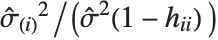 , where
  is the
  th single deletion variance.
The Durbin–Watson  ‐statistic "DurbinWatsonD" is used for testing the existence of a first-order autoregressive process. The
  ‐statistic is equivalent to
 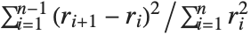 , where
  is the
  th residual.
ListPlot[lm2["CookDistances"], Filling -> 0]| "MeanPredictionBands" | confidence bands for mean predictions |
| "MeanPredictionConfidenceIntervals" | confidence intervals for the mean predictions |
| "MeanPredictionConfidenceIntervalTable" | table of confidence intervals for the mean predictions |
| "MeanPredictionConfidenceIntervalTableEntries" | unformatted array of values from the table |
| "MeanPredictionErrors" | standard errors for mean predictions |
| "PredictedResponse" | fitted values for the data |
| "SinglePredictionBands" | confidence bands based on single observations |
| "SinglePredictionConfidenceIntervals" | confidence intervals for the predicted response of single observations |
| "SinglePredictionConfidenceIntervalTable" | table of confidence intervals for the predicted response of single observations |
| "SinglePredictionConfidenceIntervalTableEntries" | unformatted array of values from the table |
| "SinglePredictionErrors" | standard errors for the predicted response of single observations |
Tabular results for confidence intervals are given by "MeanPredictionConfidenceIntervalTable" and "SinglePredictionConfidenceIntervalTable". These include the observed and predicted responses, standard error estimates, and confidence intervals for each point. Mean prediction confidence intervals are often referred to simply as confidence intervals and single prediction confidence intervals are often referred to as prediction intervals.
Mean prediction intervals give the confidence interval for the mean of the response  at fixed values of the predictors and are given by
 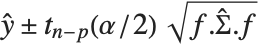 , where
  is the
  quantile of the Student
  distribution with
  degrees of freedom,
  is the vector of basis functions evaluated at fixed predictors, and
  is the estimated covariance matrix for the parameters. Single prediction intervals provide the confidence interval for predicting
  at fixed values of the predictors, and are given by
 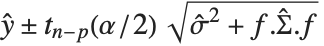 , where
  is the estimated error variance.
"MeanPredictionBands" and "SinglePredictionBands" give formulas for mean and single prediction confidence intervals as functions of the predictor variables.
lm2["MeanPredictionConfidenceIntervalTable"]lm2["MeanPredictionConfidenceIntervals", ConfidenceLevel -> .9]| "AdjustedRSquared" | |
| "AIC" | Akaike Information Criterion |
| "BIC" | Bayesian Information Criterion |
| "RSquared" | coefficient of determination |
Goodness-of-fit measures are used to assess how well a model fits or to compare models. The coefficient of determination "RSquared" is the ratio of the model sum of squares to the total sum of squares. "AdjustedRSquared" penalizes for the number of parameters in the model and is given by 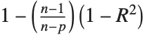 .
.
"AIC" and "BIC" are likelihood‐based goodness-of-fit measures. Both are equal to  times the log-likelihood for the model plus
  , where
  is the number of parameters to be estimated including the estimated variance. For "AIC"
  is
is  , and for "BIC"
  is
is  .
.
Generalized Linear Models
The linear model can be seen as a model with each response value  being an observation from a normal distribution with mean value
  . The generalized linear model extends to models of the form
  , with each
  assumed to be an observation from a distribution of known exponential family form with mean
  , and
, and  being an invertible function over the support of the exponential family. Models of this sort can be obtained via GeneralizedLinearModelFit.
| GeneralizedLinearModelFit[{y1,y2,…},{f1,f2,…},x] | obtain a generalized linear model with basis functions fi and a single predictor variable x |
| GeneralizedLinearModelFit[{{x11,x12,…,y1},{x21,x22,…,y2}},{f1,f2,…},{x1,x2,…}] | obtain a generalized linear model of multiple predictor variables xi |
| GeneralizedLinearModelFit[{m,v}] | obtain a generalized linear model based on a design matrix m and response vector v |
The invertible function  is called the link function and the linear combination
 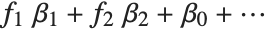 is referred to as the linear predictor. Common special cases include the linear regression model with the identity link function and Gaussian or normal exponential family distribution, logit and probit models for probabilities, Poisson models for count data, and gamma and inverse Gaussian models.
The error variance is a function of the prediction  and is defined by the distribution up to a constant
  , which is referred to as the dispersion parameter. The error variance for a fitted value
  can be written as
  , where
  is an estimate of the dispersion parameter obtained from the observed and predicted response values, and
  is the variance function associated with the exponential family evaluated at the value
  .
.
glm1 = GeneralizedLinearModelFit[Sqrt[Range[10]], x, x]glm2 = GeneralizedLinearModelFit[Sqrt[Range[10]], x, x, ExponentialFamily -> "Gamma"]Map[Normal, {glm1, glm2}]Logit and probit models are common binomial models for probabilities. The link function for the logit model is 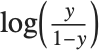 and the link for the probit model is the inverse CDF for a standard normal distribution
  . Models of this type can be fitted via GeneralizedLinearModelFit with ExponentialFamily->"Binomial" and the appropriate LinkFunction or via LogitModelFit and ProbitModelFit.
| LogitModelFit[data,funs,vars] | obtain a logit model with basis functions funs and predictor variables vars |
| LogitModelFit[{m,v}] | obtain a logit model based on a design matrix m and response vector v |
| ProbitModelFit[data,funs,vars] | obtain a probit model fit to data |
| ProbitModelFit[{m,v}] | obtain a probit model fit to a design matrix m and response vector v |
Parameter estimates are obtained via iteratively reweighted least squares with weights obtained from the variance function of the assumed distribution. Options for GeneralizedLinearModelFit include options for iteration fitting such as PrecisionGoal, options for model specification such as LinkFunction, and options for further analysis such as ConfidenceLevel.
option name | default value | |
| AccuracyGoal | Automatic | the accuracy sought |
| ConfidenceLevel | 95/100 | confidence level to use for parameters and predictions |
| CovarianceEstimatorFunction | "ExpectedInformation" | estimation method for the parameter covariance matrix |
| DispersionEstimatorFunction | Automatic | function for estimating the dispersion parameter |
| ExponentialFamily | Automatic | exponential family distribution for y |
| IncludeConstantBasis | True | whether to include a constant basis function |
| LinearOffsetFunction | None | known offset in the linear predictor |
| LinkFunction | Automatic | link function for the model |
| MaxIterations | Automatic | maximum number of iterations to use |
| NominalVariables | None | variables considered as nominal or categorical |
| PrecisionGoal | Automatic | the precision sought |
| Weights | Automatic | weights for data elements |
| WorkingPrecision | Automatic | precision used in internal computations |
Options for GeneralizedLinearModelFit.
The options for LogitModelFit and ProbitModelFit are the same as for GeneralizedLinearModelFit except that ExponentialFamily and LinkFunction are defined by the logit or probit model and so are not options to LogitModelFit and ProbitModelFit.
ExponentialFamily can be "Binomial", "Gamma", "Gaussian", "InverseGaussian", "Poisson", or "QuasiLikelihood". Binomial models are valid for responses from 0 to 1. Poisson models are valid for non-negative integer responses. Gaussian or normal models are valid for real responses. Gamma and inverse Gaussian models are valid for positive responses. Quasi-likelihood models define the distributional structure in terms of a variance function  such that the log of the quasi‐likelihood function for the
  th data point is given by
  . The variance function for a "QuasiLikelihood" model can be optionally set via ExponentialFamily->{"QuasiLikelihood", "VarianceFunction"->fun}, where fun is a pure function to be applied to fitted values.
DispersionEstimatorFunction defines a function for estimating the dispersion parameter  . The estimate
  is analogous to
  in linear and nonlinear regression models.
ExponentialFamily, IncludeConstantBasis, LinearOffsetFunction, LinkFunction, NominalVariables, and Weights all define some aspect of the model structure and optimization criterion and can only be set within GeneralizedLinearModelFit. All other options can be set either within GeneralizedLinearModelFit or passed to the FittedModel object when obtaining results and diagnostics. Options set in evaluations of FittedModel objects take precedence over settings given to GeneralizedLinearModelFit at the time of the fitting.
{glm2["ParameterConfidenceIntervals"], glm2["ParameterConfidenceIntervals", ConfidenceLevel -> .99]}| "BasisFunctions" | list of basis functions |
| "BestFit" | fitted function |
| "BestFitParameters" | parameter estimates |
| "Data" | the input data or design matrix and response vector |
| "DesignMatrix" | design matrix for the model |
| "Function" | best fit pure function |
| "LinearPredictor" | fitted linear combination |
| "Response" | response values in the input data |
"BestFitParameters" gives the parameter estimates for the basis functions. "BestFit" gives the fitted function  , and "LinearPredictor" gives the linear combination
  . "BasisFunctions" gives the list of functions
  , with
  being the constant 1 when a constant term is present in the model. "DesignMatrix" is the design or model matrix for the basis functions.
| "Deviances" | deviances |
| "DevianceTable" | deviance table |
| "DevianceTableDegreesOfFreedom" | degrees of freedom differences from the table |
| "DevianceTableDeviances" | deviance differences from the table |
| "DevianceTableEntries" | unformatted array of values from the table |
| "DevianceTableResidualDegreesOfFreedom" | residual degrees of freedom from the table |
| "DevianceTableResidualDeviances" | residual deviances from the table |
| "EstimatedDispersion" | estimated dispersion parameter |
| "NullDeviance" | deviance for the null model |
| "NullDegreesOfFreedom" | degrees of freedom for the null model |
| "ResidualDeviance" | difference between the deviance for the fitted model and the deviance for the full model |
| "ResidualDegreesOfFreedom" | difference between the model degrees of freedom and null degrees of freedom |
Deviances and deviance tables generalize the model decomposition given by analysis of variance in linear models. The deviance for a single data point is  , where
  is the log-likelihood function for the fitted model. "Deviances" gives a list of the deviance values for all data points. The sum of all deviances gives the model deviance. The model deviance can be decomposed as sums of squares, which are in an ANOVA table for linear models. The full model is the model whose predicted values are the same as the data.
glmdata = {{3.58, 1.83, 0.21}, {3.58, 4.47, 0.17}, {3.58, 3.11, 0.19}, {3.58, 4.2, 0.18}, {3.58, 2.83, 0.2}, {4.01, 2.53, 0.19}, {4.01, 3.63, 0.18}, {4.01, 3.93, 0.17}, {4.01, 4.05, 0.17}, {4.01, 1.33, 0.22}, {2.01, 3.46, 0.22}, {2.01, 1.77, 0.25}, {2.01, 2.44, 0.23}, {2.01, 2.39, 0.25}, {2.01, 3.78, 0.2}, {3.59, 3.49, 0.19}, {3.59, 3.82, 0.19}, {3.59, 3.05, 0.2}, {3.59, 4.51, 0.17}, {3.59, 3.37, 0.18}, {2.62, 1.42, 0.25}, {2.62, 3.9, 0.19}, {2.62, 2.51, 0.21}, {2.62, 4.59, 0.18}, {2.62, 4.28, 0.19}};glm3 = GeneralizedLinearModelFit[glmdata, {x, y}, {x, y}, ExponentialFamily -> "InverseGaussian"]glm3["DevianceTable"]As with sums of squares, deviances are additive. The Deviance column of the table gives the increase in the model deviance when the given basis function is added. The Residual Deviance column gives the difference between the model deviance and the deviance for the submodel containing all previous terms in the table. For large samples, the increase in deviance is approximately  distributed with degrees of freedom equal to that for the basis function in the table.
"NullDeviance" is the deviance for the null model, the constant model equal to the mean of all observed responses for models including a constant, or  if a constant term is not included.
As with "ANOVATable", a number of properties are included to extract the columns or unformatted array of entries from "DevianceTable".
| "AnscombeResiduals" | Anscombe residuals |
| "DevianceResiduals" | deviance residuals |
| "FitResiduals" | difference between actual and predicted responses |
| "LikelihoodResiduals" | likelihood residuals |
| "PearsonResiduals" | Pearson residuals |
| "StandardizedDevianceResiduals" | standardized deviance residuals |
| "StandardizedPearsonResiduals" | standardized Pearson residuals |
| "WorkingResiduals" | working residuals |
"FitResiduals" is the list of residuals, differences between the observed and predicted responses. Given the distributional assumptions, the magnitude of the residuals is expected to change as a function of the predicted response value. Various types of scaled residuals are employed in the analysis of generalized linear models.
If  and
and  are the deviance and residual for the
  th data point, the
  th deviance residual is given by
  . The
. The  th Pearson residual is defined as
  , where
  is the variance function for the exponential family distribution. Standardized deviance residuals and standardized Pearson residuals include division by
  , where
  is the
  th diagonal of the hat matrix. "LikelihoodResiduals" values combine deviance and Pearson residuals. The
  th likelihood residual is given by
  .
.
"AnscombeResiduals" provide a transformation of the residuals toward normality, so a plot of these residuals should be expected to look roughly like white noise. The  th Anscombe residual can be written as
  .
.
"WorkingResiduals" gives the residuals from the last step of the iterative fitting. The  th working residual can be obtained as
  evaluated at
  .
.
Map[ListPlot[#, Filling -> 0]&, glm3[{"FitResiduals", "AnscombeResiduals"}]]| "CorrelationMatrix" | asymptotic parameter correlation matrix |
| "CovarianceMatrix" | asymptotic parameter covariance matrix |
| "ParameterConfidenceIntervals" | parameter confidence intervals |
| "ParameterConfidenceIntervalTable" | table of confidence interval information for the fitted parameters |
| "ParameterConfidenceIntervalTableEntries" | unformatted array of values from the table |
| "ParameterConfidenceRegion" | ellipsoidal parameter confidence region |
| "ParameterTableEntries" | unformatted array of values from the table |
| "ParameterErrors" | standard errors for parameter estimates |
| "ParameterPValues" | |
| "ParameterTable" | table of fitted parameter information |
| "ParameterZStatistics" |
"CovarianceMatrix" gives the covariance between fitted parameters and is very similar to the definition for linear models. With CovarianceEstimatorFunction->"ExpectedInformation", the expected information matrix obtained from the iterative fitting is used. The matrix is  , where
  is the design matrix and
  is the diagonal matrix of weights from the final stage of the fitting. The weights include both weights specified via the Weights option and the weights associated with the distribution's variance function. With CovarianceEstimatorFunction->"ObservedInformation", the matrix is given by
  , where
  is the observed Fisher information matrix, which is the Hessian of the log‐likelihood function with respect to parameters of the model.
"CorrelationMatrix" is the associated correlation matrix for the parameter estimates. "ParameterErrors" is equivalent to the square root of the diagonal elements of the covariance matrix. "ParameterTable" and "ParameterConfidenceIntervalTable" contain information about the individual parameter estimates, tests of parameter significance, and confidence intervals. The test statistics for generalized linear models asymptotically follow normal distributions.
"CookDistances" and "HatDiagonal" extend the leverage measures from linear regression to generalized linear models. The hat matrix from which the diagonal elements are extracted is defined using the final weights of the iterative fitting.
The Cook distance measures of leverage are defined as in linear regression with standardized residuals replaced by standardized Pearson residuals. The  th Cook distance is given by
  , where
  is the
  th standardized Pearson residual.
| "AdjustedLikelihoodRatioIndex" | Ben‐Akiva and Lerman's adjusted likelihood ratio index |
| "AIC" | Akaike Information Criterion |
| "BIC" | Bayesian Information Criterion |
| "CoxSnellPseudoRSquared" | Cox and Snell's pseudo |
| "CraggUhlerPseudoRSquared" | Cragg and Uhler's pseudo |
| "EfronPseudoRSquared" | Efron's pseudo |
| "LikelihoodRatioIndex" | McFadden's likelihood ratio index |
| "LikelihoodRatioStatistic" | likelihood ratio |
| "LogLikelihood" | log likelihood for the fitted model |
| "PearsonChiSquare" | Pearson's |
"LogLikelihood" is the log‐likelihood for the fitted model. "AIC" and "BIC" are penalized log‐likelihood measures  , where
  is the log‐likelihood for the fitted model,
  is the number of parameters estimated including the dispersion parameter, and
  is
is  for "AIC" and
  for "BIC" for a model of
  data points. "LikelihoodRatioStatistic" is given by
  , where
  is the log‐likelihood for the null model.
A number of the goodness-of-fit measures generalize  from linear regression as either a measure of explained variation or as a likelihood‐based measure. "CoxSnellPseudoRSquared" is given by
  . "CraggUhlerPseudoRSquared" is a scaled version of Cox and Snell's measure
  . "LikelihoodRatioIndex" involves the ratio of log‐likelihoods
  , and "AdjustedLikelihoodRatioIndex" adjusts by penalizing for the number of parameters
  . "EfronPseudoRSquared" uses the sum of squares interpretation of
  and is given as
  , where
  is the
  th residual and
  is the mean of the responses
  .
.
Nonlinear Models
A nonlinear least-squares model is an extension of the linear model where the model need not be a linear combination of basis function. The errors are still assumed to be independent and normally distributed. Models of this type can be fitted using the NonlinearModelFit function.
| NonlinearModelFit[{y1,y2,…},form,{β1,…},x] | obtain a nonlinear model of the function form with parameters βi a single parameter predictor variable x |
| NonlinearModelFit[{{x11,…,y1},{x21,…,y2}},form,{β1,…},{x1,…}] | obtain a nonlinear model as a function of multiple predictor variables xi |
| NonlinearModelFit[data,{form,cons},{β1,…},{x1,…}] | obtain a nonlinear model subject to the constraints cons |
Nonlinear models have the form  , where
  is the fitted or predicted value, the
  are parameters to be fitted, and the
  are predictor variables. As with any nonlinear optimization problem, a good choice of starting values for the parameters may be necessary. Starting values can be given using the same parameter specifications as for FindFit.
nlm = NonlinearModelFit[Array[Sqrt, 20], Log[a + b x], {a, b}, x]option name | default value | |
| AccuracyGoal | Automatic | the accuracy sought |
| ConfidenceLevel | 95/100 | confidence level to use for parameters and predictions |
| EvaluationMonitor | None | expression to evaluate whenever expr is evaluated |
| MaxIterations | Automatic | maximum number of iterations to use |
| Method | Automatic | method to use |
| PrecisionGoal | Automatic | the precision sought |
| StepMonitor | None | the expression to evaluate whenever a step is taken |
| VarianceEstimatorFunction | Automatic | function for estimating the error variance |
| Weights | Automatic | weights for data elements |
| WorkingPrecision | Automatic | precision used in internal computations |
Options for NonlinearModelFit.
General numeric options such as AccuracyGoal, Method, and WorkingPrecision are the same as for FindFit.
The Weights option specifies weight values for weighted nonlinear regression. The optimal fit is for a weighted sum of squared errors.
All other options can be relevant to computation of results after the initial fitting. They can be set within NonlinearModelFit for use in the fitting and to specify the default settings for results obtained from the FittedModel object. These options can also be set within an already constructed FittedModel object to override the option values originally given to NonlinearModelFit.
| "BestFit" | fitted function |
| "BestFitParameters" | parameter estimates |
| "Data" | the input data |
| "Function" | best fit pure function |
| "Response" | response values in the input data |
Basic properties of the data and fitted function for nonlinear models behave like the same properties for linear and generalized linear models with the exception that "BestFitParameters" returns a rule as is done for the result of FindFit.
nlm[{"BestFit", "BestFitParameters"}]Many diagnostics for nonlinear models extend or generalize concepts from linear regression. These extensions often rely on linear approximations or large sample approximations.
| "FitResiduals" | difference between actual and predicted responses |
| "StandardizedResiduals" | fit residuals divided by the standard error for each residual |
| "StudentizedResiduals" | fit residuals divided by single deletion error estimates |
As in linear regression, "FitResiduals" gives the differences between the observed and fitted values  , and "StandardizedResiduals" and "StudentizedResiduals" are scaled forms of these differences.
The  th standardized residual is
  , where
  is the estimated error variance,
  is the
  th diagonal element of the hat matrix, and
  is the weight for the
  th data point, and the
  th studentized residual is obtained by
  replacing with the
  th single deletion variance
  . For nonlinear models a first-order approximation is used for the design matrix, which is needed to compute the hat matrix.
| "ANOVATable" | analysis of variance table |
| "ANOVATableDegreesOfFreedom" | degrees of freedom from the ANOVA table |
| "ANOVATableEntries" | unformatted array of values from the table |
| "ANOVATableMeanSquares" | mean square errors from the table |
| "ANOVATableSumsOfSquares" | sums of squares from the table |
| "EstimatedVariance" | estimate of the error variance |
"ANOVATable" provides a decomposition of the variation in the data attributable to the fitted function and to the errors or residuals.
nlm["ANOVATable"]The uncorrected total sums of squares gives the sum of squared responses, while the corrected total gives the sum of squared differences between the responses and their mean value.
| "CorrelationMatrix" | asymptotic parameter correlation matrix |
| "CovarianceMatrix" | asymptotic parameter covariance matrix |
| "ParameterBias" | estimated bias in the parameter estimates |
| "ParameterConfidenceIntervals" | parameter confidence intervals |
| "ParameterConfidenceIntervalTable" | table of confidence interval information for the fitted parameters |
| "ParameterConfidenceIntervalTableEntries" | unformatted array of values from the table |
| "ParameterConfidenceRegion" | ellipsoidal parameter confidence region |
| "ParameterErrors" | standard errors for parameter estimates |
| "ParameterPValues" | |
| "ParameterTable" | table of fitted parameter information |
| "ParameterTableEntries" | unformatted array of values from the table |
| "ParameterTStatistics" |
"CovarianceMatrix" gives the approximate covariance between fitted parameters. The matrix is  , where
  is the variance estimate,
  is the design matrix for the linear approximation to the model, and
  is the diagonal matrix of weights. "CorrelationMatrix" is the associated correlation matrix for the parameter estimates. "ParameterErrors" is equivalent to the square root of the diagonal elements of the covariance matrix.
"ParameterTable" and "ParameterConfidenceIntervalTable" contain information about the individual parameter estimates, tests of parameter significance, and confidence intervals obtained using the error estimates.
| "CurvatureConfidenceRegion" | confidence region for curvature diagnostics |
| "FitCurvatureTable" | table of curvature diagnostics |
| "FitCurvatureTableEntries" | unformatted array of values from the table |
| "MaxIntrinsicCurvature" | measure of maximum intrinsic curvature |
| "MaxParameterEffectsCurvature" | measure of maximum parameter effects curvature |
The first-order approximation used for many diagnostics is equivalent to the model being linear in the parameters. If the parameter space near the parameter estimates is sufficiently flat, the linear approximations and any results that rely on first-order approximations can be deemed reasonable. Curvature diagnostics are used to assess whether the approximate linearity is reasonable. "FitCurvatureTable" is a table of curvature diagnostics.
"MaxIntrinsicCurvature" and "MaxParameterEffectsCurvature" are scaled measures of the normal and tangential curvatures of the parameter spaces at the best-fit parameter values. "CurvatureConfidenceRegion" is a scaled measure of the radius of curvature of the parameter space at the best-fit parameter values. If the normal and tangential curvatures are small relative to the value of the "CurvatureConfidenceRegion", the linear approximation is considered reasonable. Some rules of thumb suggest comparing the values directly, while others suggest comparing with half the "CurvatureConfidenceRegion".
nlm["FitCurvatureTable"]| "HatDiagonal" | diagonal elements of the hat matrix |
| "SingleDeletionVariances" | list of variance estimates with the |
The hat matrix is the matrix  such that
  , where
  is the observed response vector and
  is the predicted response vector. "HatDiagonal" gives the diagonal elements of the hat matrix. As with other properties,
  uses the design matrix for the linear approximation to the model.
The  th element of "SingleDeletionVariances" is equivalent to
  , where
  is the number of data points,
  is the number of parameters,
  is the
  th hat diagonal,
  is the variance estimate for the full dataset, and
  is the
  th residual.
| "MeanPredictionBands" | confidence bands for mean predictions |
| "MeanPredictionConfidenceIntervals" | confidence intervals for the mean predictions |
| "MeanPredictionConfidenceIntervalTable" | table of confidence intervals for the mean predictions |
| "MeanPredictionConfidenceIntervalTableEntries" | unformatted array of values from the table |
| "MeanPredictionErrors" | standard errors for mean predictions |
| "PredictedResponse" | fitted values for the data |
| "SinglePredictionBands" | confidence bands based on single observations |
| "SinglePredictionConfidenceIntervals" | confidence intervals for the predicted response of single observations |
| "SinglePredictionConfidenceIntervalTable" | table of confidence intervals for the predicted response of single observations |
| "SinglePredictionConfidenceIntervalTableEntries" | unformatted array of values from the table |
| "SinglePredictionErrors" | standard errors for the predicted response of single observations |
Tabular results for confidence intervals are given by "MeanPredictionConfidenceIntervalTable" and "SinglePredictionConfidenceIntervalTable". These results are analogous to those for linear models obtained via LinearModelFit, again with first-order approximations used for the design matrix.
{fit[x_], mp[x_]} = nlm[{"BestFit", "MeanPredictionBands"}]Plot[{fit[x], mp[x]}, {x, 1, 20}]| "AdjustedRSquared" | |
| "AIC" | Akaike Information Criterion |
| "BIC" | Bayesian Information Criterion |
| "RSquared" | coefficient of determination |
"AdjustedRSquared", "AIC", "BIC", and "RSquared" are all direct extensions of the measures as defined for linear models. The coefficient of determination "RSquared" is  , where
  is the residual sum of squares and
  is the uncorrected total sum of squares. The coefficient of determination does not have the same interpretation as the percentage of explained variation in nonlinear models as it does in linear models because the sum of squares for the model and for the residuals do not necessarily sum to the total sum of squares. "AdjustedRSquared" penalizes for the number of parameters in the model and is given by
  .
.
"AIC" and "BIC" are equal to  times the log-likelihood for the model plus
  , where
  is the number of parameters to be estimated including the estimated variance. For "AIC"
  is
is  , and for "BIC"
  is
is  .
.
In many kinds of numerical computations, it is convenient to introduce approximate functions. Approximate functions can be thought of as generalizations of ordinary approximate real numbers. While an approximate real number gives the value to a certain precision of a single numerical quantity, an approximate function gives the value to a certain precision of a quantity which depends on one or more parameters. The Wolfram Language uses approximate functions, for example, to represent numerical solutions to differential equations obtained with NDSolve, as discussed in "Numerical Differential Equations".
Approximate functions in the Wolfram Language are represented by InterpolatingFunction objects. These objects work like the pure functions discussed in "Pure Functions". The basic idea is that when given a particular argument, an InterpolatingFunction object finds the approximate function value that corresponds to that argument.
The InterpolatingFunction object contains a representation of the approximate function based on interpolation. Typically it contains values and possibly derivatives at a sequence of points. It effectively assumes that the function varies smoothly between these points. As a result, when you ask for the value of the function with a particular argument, the InterpolatingFunction object can interpolate to find an approximation to the value you want.
| Interpolation[{f1,f2,…}] | construct an approximate function with values fi at successive integers |
| Interpolation[{{x1,f1},{x2,f2},…}] | |
construct an approximate function with values fi at points xi | |
Table[{x, Sin[x]}, {x, 0, 2, 0.25}]sin = Interpolation[%]sin[0.25]sin[0.3]Sin[0.3]You can work with approximate functions much as you would with any other Wolfram Language functions. You can plot approximate functions, or perform numerical operations such as integration or root finding.
sin[x]NIntegrate[sin[x] ^ 2, {x, 0, Pi / 2}]NIntegrate[Sin[x] ^ 2, {x, 0, Pi / 2}]Plot[sin[x], {x, 0, 2}]If you differentiate an approximate function, the Wolfram Language will return another approximate function that represents the derivative.
sin'[Pi / 6]N[Cos[Pi / 6]]InterpolatingFunction objects contain all the information the Wolfram Language needs about approximate functions. In standard Wolfram Language output format, however, only the part that gives the domain of the InterpolatingFunction object is printed explicitly. The lists of actual parameters used in the InterpolatingFunction object are shown only in iconic form.
In standard output format, the only parts of an InterpolatingFunction object printed explicitly are its domain and output type:
sinIf you ask for a value outside of the domain, the Wolfram Language prints a warning, then uses extrapolation to find a result:
sin[3]The more information you give about the function you are trying to approximate, the better the approximation the Wolfram Language constructs can be. You can, for example, specify not only values of the function at a sequence of points, but also derivatives.
| Interpolation[{{{x1},f1,df1,ddf1,…},…}] | |
construct an approximate function with specified derivatives at points xi | |
sind = Interpolation[Table[{{x}, Sin[x], Cos[x]}, {x, 0, 2, 0.25}]]sind'[Pi / 6]Interpolation works by fitting polynomial curves between the points you specify. You can use the option InterpolationOrder to specify the degree of these polynomial curves. The default setting is InterpolationOrder->3, yielding cubic curves.
tab = Table[{x, Cos[x]}, {x, 0, 6}];Interpolation[tab, InterpolationOrder -> 1]Plot[%[x], {x, 0, 6}]With the default setting InterpolationOrder->3, cubic curves are used, and the function looks smooth:
Plot[Evaluate[Interpolation[tab]][x], {x, 0, 6}]Increasing the setting for InterpolationOrder typically leads to smoother approximate functions. However, if you increase the setting too much, spurious wiggles may develop.
| ListInterpolation[{{f11,f12,…},{f21,…},…}] | |
construct an approximate function from a two‐dimensional grid of values at integer points | |
| ListInterpolation[list,{{xmin,xmax},{ymin,ymax}}] | |
assume the values are from an evenly spaced grid with the specified domain | |
| ListInterpolation[list,{{x1,x2,…},{y1,y2,…}}] | |
assume the values are from a grid with the specified grid lines | |
ListInterpolation[Table[1.5 / (x ^ 2 + y ^ 3), {x, 10}, {y, 15}]]%[6.5, 7.2]tab = Table[1.5 / (x ^ 2 + y ^ 3), {x, 5.5, 7.2, .2}, {y, 2.3, 8.9, .1}];ListInterpolation[tab, {{5.5, 7.2}, {2.3, 8.9}}]ListInterpolation works for arrays of any dimension, and in each case it produces an InterpolatingFunction object which takes the appropriate number of arguments.
ListInterpolation[Array[#1 ^ 2 + #2 ^ 2 - #3 ^ 2&, {10, 10, 10}]]The resulting InterpolatingFunction object takes three arguments:
%[3.4, 7.8, 2.6]The Wolfram Language can handle not only purely numerical approximate functions, but also ones which involve symbolic parameters.
sfun = ListInterpolation[{1 + a, 2, 3, 4 + b, 5}];sfun[2.2]//SimplifyWith the default setting for InterpolationOrder used, the value at this point no longer depends on a:
sfun[3.8]//SimplifyIn working with approximate functions, you can quite often end up with complicated combinations of InterpolatingFunction objects. You can always tell the Wolfram Language to produce a single InterpolatingFunction object valid over a particular domain by using FunctionInterpolation.
This generates a new InterpolatingFunction object valid in the domain 0 to 1:
FunctionInterpolation[x + sin[x ^ 2], {x, 0, 1}]This generates a nested InterpolatingFunction object:
ListInterpolation[{3, 4, 5, sin[a], 6}][4]FunctionInterpolation[x ^ 2 + %, {x, 1, 3}, {a, 0, 1.5}]| FunctionInterpolation[expr,{x,xmin,xmax}] | |
construct an approximate function by evaluating expr with x ranging from xmin to xmax | |
| FunctionInterpolation[expr,{x,xmin,xmax},{y,ymin,ymax},…] | |
construct a higher‐dimensional approximate function | |
A common operation in analyzing various kinds of data is to find the discrete Fourier transform (or spectrum) of a list of values. The idea is typically to pick out components of the data with particular frequencies or ranges of frequencies.
| Fourier[{u1,u2,…,un}] | discrete Fourier transform |
| InverseFourier[{v1,v2,…,vn}] | inverse discrete Fourier transform |
{-1, -1, -1, -1, 1, 1, 1, 1}Fourier[%]InverseFourier[%]Fourier works whether or not your list of data has a length which is a power of two:
Fourier[{1, -1, 1}]data = Table[N[Sin[30 2 Pi n / 200] + (RandomReal[] - 1 / 2)], {n, 200}];ListLinePlot[data]The discrete Fourier transform, however, shows a strong peak at  , and a symmetric peak at
  , reflecting the frequency component of the original signal near
  :
:
ListLinePlot[Abs[Fourier[data]], PlotRange -> All]In the Wolfram Language, the discrete Fourier transform  of a list
  of length
  is by default defined to be
  . Notice that the zero frequency term appears at position 1 in the resulting list.
In different scientific and technical fields different conventions are often used for defining discrete Fourier transforms. The option FourierParameters allows you to choose any of these conventions you want.
common convention | setting | discrete Fourier transform | inverse discrete Fourier transform |
Wolfram Language default | {0,1} | ||
data analysis | {-1,1} | ||
signal processing | {1,-1} | ||
general case | {a,b} |
Typical settings for FourierParameters with various conventions.
| Fourier[{{u11,u12,…},{u21,u22,…},…}] | |
two‐dimensional discrete Fourier transform | |
The Wolfram Language can find discrete Fourier transforms for data in any number of dimensions. In  dimensions, the data is specified by a list nested
  levels deep. Two‐dimensional discrete Fourier transforms are often used in image processing.
One issue with the usual discrete Fourier transform for real data is that the result is complex-valued. There are variants of real discrete Fourier transforms that have real results. The Wolfram Language has commands for computing the discrete cosine transform and the discrete sine transform.
| FourierDCT[list] | Fourier discrete cosine transform of a list of real numbers |
| FourierDST[list] | Fourier discrete sine transform of a list of real numbers |
pulse = {-1, -1, -1, -1, -1, 1, 1, 1, 1, 1}FourierDCT[pulse]FourierDST[pulse]There are four types each of Fourier discrete sine and cosine transforms typically in use, denoted by number or sometimes roman numeral as in "DCTII" for the discrete cosine transform of type 2.
| FourierDCT[list,m] | Fourier discrete cosine transform of type m |
| FourierDST[list,m] | Fourier discrete sine transform of type m |
The Wolfram Language does not need InverseFourierDCT or InverseFourierDST functions because FourierDCT and FourierDST are their own inverses when used with the appropriate type. The inverse transforms for types 1, 2, 3, 4 are types 1, 3, 2, 4, respectively.
FourierDCT[FourierDCT[pulse, 2], 3]data = Table[ArcTan[x - 100], {x, 1., 200.}];
ListLinePlot[data]dct = FourierDCT[data];
ListLinePlot[dct, PlotRange -> All]Reconstruct the front from only the first 20 modes (1/10 of the original data size). The oscillations are a consequence of the truncation and are known to show up in image processing applications as well:
tdata = FourierDCT[PadRight[Take[dct, 20], 200, 0], 3];
ListLinePlot[{data, tdata}]Convolution and correlation are central to many kinds of operations on lists of data. They are used in such areas as signal and image processing, statistical data analysis, and approximations to partial differential equations, as well as operations on digit sequences and power series.
In both convolution and correlation the basic idea is to combine a kernel list with successive sublists of a list of data. The convolution of a kernel  with a list
  has the general form
  , while the correlation has the general form
  .
.
| ListConvolve[kernel,list] | form the convolution of kernel with list |
| ListCorrelate[kernel,list] | form the correlation of kernel with list |
ListConvolve[{x, y}, {a, b, c, d, e}]ListCorrelate[{x, y}, {a, b, c, d, e}]In this case reversing the kernel gives exactly the same result as ListConvolve:
ListCorrelate[{y, x}, {a, b, c, d, e}]ListCorrelate[{-1, 1}, {a, b, c, d, e}]In forming sublists to combine with a kernel, there is always an issue of what to do at the ends of the list of data. By default, ListConvolve and ListCorrelate never form sublists which would "overhang" the ends of the list of data. This means that the output you get is normally shorter than the original list of data.
ListCorrelate[{1, 1, 1}, Range[6]]In practice one often wants to get output that is as long as the original list of data. To do this requires including sublists that overhang one or both ends of the list of data. The additional elements needed to form these sublists must be filled in with some kind of "padding". By default, the Wolfram Language takes copies of the original list to provide the padding, thus effectively treating the list as being cyclic.
| ListCorrelate[kernel,list] |
do not allow overhangs on either side (result shorter than
list
)
|
| ListCorrelate[kernel,list,1] |
allow an overhang on the right (result same length as
list
)
|
| ListCorrelate[kernel,list,-1] |
allow an overhang on the left (result same length as
list
)
|
| ListCorrelate[kernel,list,{-1,1}] |
allow overhangs on both sides (result longer than
list
)
|
| ListCorrelate[kernel,list,{kL,kR}] | allow particular overhangs on left and right |
ListCorrelate[{x, y}, {a, b, c, d}]ListCorrelate[{x, y}, {a, b, c, d}, 1]Now the first term of the first element and the last term of the last element both involve wraparound:
ListCorrelate[{x, y}, {a, b, c, d}, {-1, 1}]In the general case ListCorrelate[kernel,list,{kL,kR}] is set up so that in the first element of the result, the first element of list appears multiplied by the element at position kL in kernel, and in the last element of the result, the last element of list appears multiplied by the element at position kR in kernel. The default case in which no overhang is allowed on either side thus corresponds to ListCorrelate[kernel,list,{1,-1}].
With a kernel of length 3, alignments {-1,2} always make the first and last elements of the result the same:
ListCorrelate[{x, y, z}, {a, b, c, d}, {-1, 2}]For many kinds of data, it is convenient to assume not that the data is cyclic, but rather that it is padded at either end by some fixed element, often 0, or by some sequence of elements.
| ListCorrelate[kernel,list,klist,p] | pad with element p |
| ListCorrelate[kernel,list,klist,{p1,p2,…}] | |
pad with cyclic repetitions of the pi | |
| ListCorrelate[kernel,list,klist,list] | pad with cyclic repetitions of the original data |
ListCorrelate[{x, y}, {a, b, c, d}, {-1, 1}, p]ListCorrelate[{x, y}, {a, b, c, d}, {-1, 1}, 0]When the padding is indicated by {p,q}, the list {a,b,c} overlays {…,p,q,p,q,…} with a p aligned under the a:
ListCorrelate[{x, y, z}, {a, b, c}, {-1, 1}, {p, q}]Different choices of kernel allow ListConvolve and ListCorrelate to be used for different kinds of computations.
ListCorrelate[{1, 1, 1} / 3, {a, b, c, d, e}]kern = Table[Exp[-n ^ 2 / 100] / Sqrt[2. Pi], {n, -10, 10}];data = Table[BesselJ[1, x] + 0.2 RandomReal[], {x, 0, 10, .1}];ListPlot[data]ListConvolve[kern, data];ListPlot[%]ListConvolve[{a, b, c}, {u, v, w}, {1, -1}, 0]The result corresponds exactly with the coefficients in the expanded form of this product of polynomials:
Expand[(a + b x + c x ^ 2)(u + v x + w x ^ 2)]g = ReadList["ExampleData/fish.data", Number, RecordLists -> True];Graphics[Raster[g]]ListConvolve[{{1, 1, 1}, {1, -8, 1}, {1, 1, 1}}, g];Graphics[Raster[%]]Cellular automata provide a convenient way to represent many kinds of systems in which the values of cells in an array are updated in discrete steps according to a local rule.
| CellularAutomaton[rnum,init,t] | evolve rule rnum from init for t steps |
CellularAutomaton[30, {0, 0, 0, 1, 0, 0, 0}, 4]ArrayPlot[CellularAutomaton[30, RandomInteger[1, 250], 100]]| {a1,a2,…} | explicit list of values ai |
| {{a1,a2,…},b} | values ai superimposed on a b background |
| {{a1,a2,…},blist} | values ai superimposed on a background of repetitions of blist |
| {{{{a11,a12,…},{d1}},…},blist} | values aij at offsets di |
If you give an explicit list of initial values, CellularAutomaton will take the elements in this list to correspond to all the cells in the system, arranged cyclically.
CellularAutomaton[30, {1, 0, 0, 0, 0}, 1]It is often convenient to set up initial conditions in which there is a small "seed" region, superimposed on a constant "background". By default, CellularAutomaton automatically fills in enough background to cover the size of the pattern that can be produced in the number of steps of evolution you specify.
ArrayPlot[CellularAutomaton[30, {{1}, 0}, 100]]This shows rule 30 evolving from an initial condition consisting of a {1,1} seed on a background of repeated {1,0,1,1} blocks:
ArrayPlot[CellularAutomaton[30, {{1, 1}, {1, 0, 1, 1}}, 100]]Particularly in studying interactions between structures, you may sometimes want to specify initial conditions for cellular automata in which certain blocks are placed at particular offsets.
ArrayPlot[CellularAutomaton[30, {{{{1}, {-40}}, {{1}, {40}}}, 0}, 100]]| n | |
| {n,k} | general nearest‐neighbor rule with k colors |
| {n,k,r} | general rule with k colors and range r |
| {n,{k,1}} | k‐color nearest‐neighbor totalistic rule |
| {n,{k,1},r} | k‐color range-r totalistic rule |
| {n,{k,{wt1,wt2,…}},r} | rule in which neighbor i is assigned weight wti |
| {n,kspec,{{off1},{off2},…,{offs}}} | rule with neighbors at specified offsets |
| {lhs1->rhs1,lhs2->rhs2,…} | explicit replacements for lists of neighbors |
| {fun,{},rspec} | rule obtained by applying function fun to each neighbor list |
In the simplest cases, a cellular automaton allows k possible values or "colors" for each cell, and has rules that involve up to r neighbors on each side. The digits of the "rule number" n then specify what the color of a new cell should be for each possible configuration of the neighborhood.
CellularAutomaton[30, {1, 1, 0}, 1]Tuples[{1, 0}, 3]Map[CellularAutomaton[30, #, 1][[2, 2]]&, %]FromDigits[%, 2]ArrayPlot[CellularAutomaton[{921408, 3, 1}, {{1}, 0}, 100]]For a general cellular automaton rule, each digit of the rule number specifies what color a different possible neighborhood of  cells should yield. To find out which digit corresponds to which neighborhood, one effectively treats the cells in a neighborhood as digits in a number. For an
  cellular automaton, the number is obtained from the list of elements neig in the neighborhood by neig.{k^2,k,1}.
It is sometimes convenient to consider totalistic cellular automata, in which the new value of a cell depends only on the total of the values in its neighborhood. One can specify totalistic cellular automata by rule numbers or "codes" in which each digit refers to neighborhoods with a given total value, obtained for example from neig.{1,1,1}.
In general, CellularAutomaton allows one to specify rules using any sequence of weights. Another choice sometimes convenient is {k,1,k}, which yields outer totalistic rules.
ArrayPlot[CellularAutomaton[{867, {3, 1}, 1}, {{1}, 0}, 100]]Rules with range  involve all cells with offsets
  through
  . Sometimes it is convenient to think about rules that involve only cells with specific offsets. You can do this by replacing a single
  with a list of offsets.
Any  cellular automaton rule can be thought of as corresponding to a Boolean function. In the simplest case, basic Boolean functions like And or Nor take two arguments. These are conveniently specified in a cellular automaton rule as being at offsets {{0},{1}}. Note that for compatibility with handling higher‐dimensional cellular automata, offsets must always be given in lists, even for one‐dimensional cellular automata.
This generates the truth table for 2‐cell‐neighborhood rule number 7, which turns out to be the Boolean function Nand:
Map[CellularAutomaton[{7, 2, {{0}, {1}}}, #, 1][[2, 2]]&, {{1, 1}, {1, 0}, {0, 1}, {0, 0}}]Rule numbers provide a highly compact way to specify cellular automaton rules. But sometimes it is more convenient to specify rules by giving an explicit function that should be applied to each possible neighborhood.
ArrayPlot[CellularAutomaton[{Mod[Apply[Plus, #], 4]&, {}, 1}, {{1}, 0}, 100]]ArrayPlot[CellularAutomaton[{Mod[Total[#] + #2, 4]&, {}, 1}, {{1}, 0}, 100]]ArrayPlot[CellularAutomaton[{Mod[1 / 2 Apply[Plus, #], 1]&, {}, 1}, {{1}, 0}, 100]]Simplify[CellularAutomaton[{Mod[Apply[Plus, #], 2]&, {}, 1}, {{a}, 0}, 2], a ∈ Integers]| CellularAutomaton[rnum,init,t] | evolve for t steps, keeping all steps |
| CellularAutomaton[rnum,init,{{t}}] | evolve for t steps, keeping only the last step |
| CellularAutomaton[rnum,init,{spect}] | keep only steps specified by spect |
| CellularAutomaton[rnum,init] |
evolve rule for one step, giving only the last step
|
CellularAutomaton[30, {{1}, 0}, {{5}}]CellularAutomaton[30, {{1}, 0}, {{4, 5}}]CellularAutomaton[30, {0, 0, 1, 0, 0}]The step specification spect works very much like taking elements from a list with Take. One difference, though, is that the initial condition for the cellular automaton is considered to be step 0. Note that any step specification of the form {…} must be enclosed in an additional list.
ArrayPlot[CellularAutomaton[30, {{1}, 0}, {{0, 100, 2}}]]| CellularAutomaton[rnum,init,t] |
keep all steps, and all relevant cells
|
| CellularAutomaton[rnum,init,{spect,specx}] | |
keep only specified steps and cells | |
Much as you can specify which steps to keep in a cellular automaton evolution, so also you can specify which cells to keep. If you give an initial condition such as {{a1,a2,…},blist}, then rd is taken to have offset 0 for the purpose of specifying which cells to keep.
| All | all cells that can be affected by the specified initial condition |
| Automatic |
all cells in the region that differs from the background (default)
|
| 0 | cell aligned with beginning of aspec |
| x | cells at offsets up to x on the right |
| -x | cells at offsets up to x on the left |
| {x} | cell at offset x to the right |
| {-x} | cell at offset x to the left |
| {x1,x2} | cells at offsets x1 through x2 |
| {x1,x2,dx} | cells x1, x1+dx, … |
ArrayPlot[CellularAutomaton[30, {{1}, 0}, {100, {-20, 100}}]]CellularAutomaton[30, {{1}, 0}, {20, {0}}]If you give an initial condition such as {{a1,a2,…},blist}, then CellularAutomaton will always effectively do the cellular automaton as if there were an infinite number of cells. By using a specx such as {x1,x2} you can tell CellularAutomaton to include only cells at specific offsets x1 through x2 in its output. CellularAutomaton by default includes cells out just far enough that their values never simply stay the same as in the background blist.
In general, given a cellular automaton rule with range  , cells out to distance
  on each side could in principle be affected in the evolution of the system. With specx being All, all these cells are included; with the default setting of Automatic, cells whose values effectively stay the same as in blist are trimmed off.
ArrayPlot[CellularAutomaton[225, {{1}, 0}, 100]]Using All for specx includes all cells that could be affected by a cellular automaton with this range:
ArrayPlot[CellularAutomaton[225, {{1}, 0}, {100, All}]]CellularAutomaton generalizes quite directly to any number of dimensions. Above two dimensions, however, totalistic and other special types of rules tend to be more useful, since the number of entries in the rule table for a general rule rapidly becomes astronomical.
| {n,k,{r1,r2,…,rd}} | |
| {n,{k,1},{1,1}} | two‐dimensional 9‐neighbor totalistic rule |
| {n,{k,{{0,1,0},{1,1,1},{0,1,0}}},{1,1}} | |
two‐dimensional 5‐neighbor totalistic rule | |
| {n,{k,{{0,k,0},{k,1,k},{0,k,0}}},{1,1}} | |
two‐dimensional 5‐neighbor outer totalistic rule | |
This is the rule specification for the two‐dimensional 9‐neighbor totalistic cellular automaton with code 797:
code797 = {797, {2, 1}, {1, 1}};CellularAutomaton[code797, {{{1}}, 0}, 1]ArrayPlot[First[CellularAutomaton[code797, {{{1}}, 0},
{{70}}]]]ArrayPlot[Map[First,
CellularAutomaton[code797, {{{1}}, 0},
{70, {0}, All}]]]