



ListDensityPlot3D
ListDensityPlot3D[farr]
値 farr の配列から平滑化密度プロットを生成する.
ListDensityPlot3D[{{x1,y1,z1,f1},…,{xn,yn,zn,fn}}]
指定された点{xi,yi,zi}における値 fiの密度プロットを生成する.
詳細とオプション
- ListDensityPlot3Dはボリューム地図としても知られている.
- ListDensityPlot3Dは与えられたデータを関数
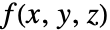 に与え,次に値を色
 と不透明度
 に個別にマップする.
- 不透明度関数
 は,通常,ある範囲の値を可視化し他の値を不可視にするために使われる.
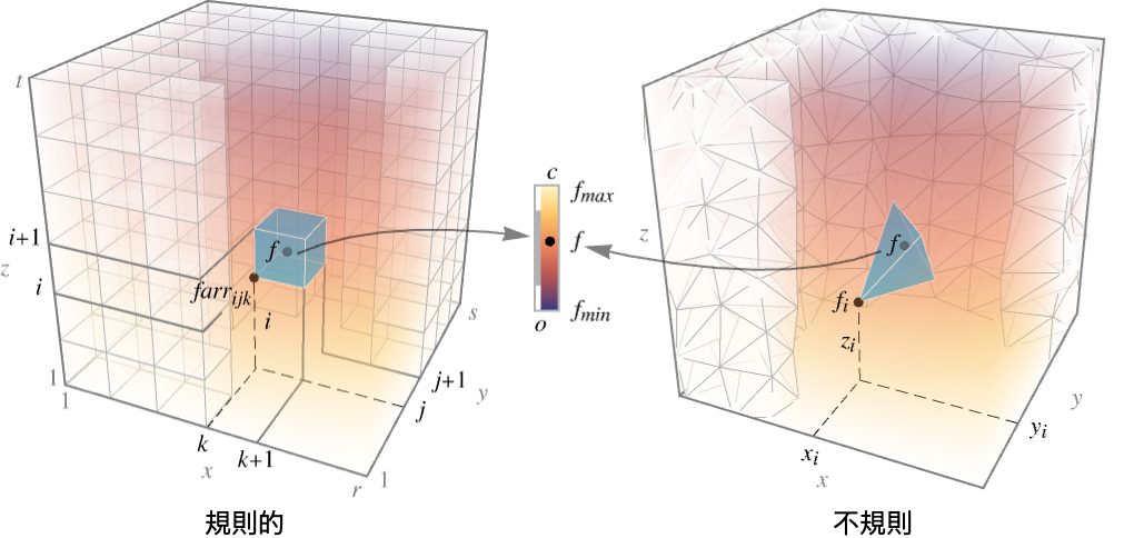
- 規則的なデータについては,関数
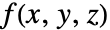 は
 で値 farr[[i,j,k]]を持つ.
- 不規則データについては,
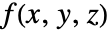 は
 で値 fiを持つ.
- 以下のプロットは集合
 を可視化する.ただし,
 は色関数で
 は不透明度の関数であり領域 reg は規則的なデータについてはデカルト積
 ,不規則データについては{{x1,y1,z1},…,{xn,yn,zn}}の凸包である.
- farr は実数配列でなければならない.farr が実数ではない位置は不透明に描画される.
- ListDensityPlot3D[Tabular[…]cspec]は,列指定 cspec を使って表オブジェクトから値を抽出し,これをプロットする.
- 次は,表データのプロットに使用可能な列指定 cspec の形式である.
-
{colx,coly,colz,colf} 列 f と列 x, y, z をプロットする - ListDensityPlot3Dは,色の変化を与えるために,値を線形に補間する.
- ListDensityPlot3Dは,主に連続した値を対象としている.ArrayPlot3Dは純粋に離散的な値を対象としている.
- ListDensityPlot3D には,Graphics3Dと同じオプションに以下の追加・変更を加えたものを使うことができる. [全オプションのリスト]
-
Axes True 軸を描くかどうか BoxRatios {1,1,1} 3D境界ボックス比 ColorFunction Automatic プロットにどのように彩色するか ColorFunctionScaling True ColorFunctionの引数をスケールするかどうか DataRange Automatic 仮定する x,y,z の値の範囲 MaxPlotPoints Automatic 含める点の最大数 OpacityFunction Automatic 各点の不透明度をどのように計算するか OpacityFunctionScaling True OpacityFunctionの引数をスケールするかどうか PerformanceGoal $PerformanceGoal パフォーマンスのどの面について最適化するか PlotLegends None 色勾配の凡例 PlotRange {Full,Full,Full,Automatic} 含める f あるいは他の値の範囲 PlotTheme $PlotTheme プロットの全体的なテーマ RegionFunction (True&) 点が含まれるかどうかをどのように決定するか ScalingFunctions None 個々の座標のスケール方法 TargetUnits Automatic 使用する所望の単位 - ColorFunctionおよびOpacityFunctionには,デフォルトで,f のスケールされた値による1つの引数が与えられる.
- OpacityFunctionのよく使われる設定
-
Automatic 自動的に決定 None 不透明度関数は使わない.完全に不透明 α 一定の不透明度 Opacity[α] Interval[…] 区間内の値をより不透明にする "Image3D" Image3Dで使われるデフォルトの不透明度関数 func 一般的な不透明度関数 - RegionFunctionに与えられる引数は,x,y,z,f である.
- DataRange->{{xmin,xmax},{ymin,ymax},{zmin,zmax}}の設定は,入力として f 値のみの array が与えられた場合に仮定すべき x,y,z の各座標範囲を指定する.
- 次元{r,s,t}の farr については,設定DataRangeAutomaticはDataRange{{1,r},{1,s},{1,t}}に等しい.
- 次は,ScalingFunctionsの可能な設定である.
-
{sx,sy,sz} x,y,z の各軸をスケールする - 次は,よく使われる組込みのスケーリング関数 s である.
-
"Log" 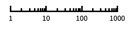
自動目盛ラベル付きの対数スケール "Log10" 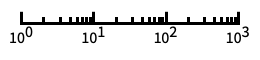
10のベキ乗に目盛が付いた,10を底とする対数スケール "SignedLog" 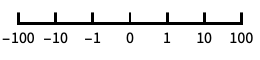
0と負の数を含む対数に似たスケール "Reverse" 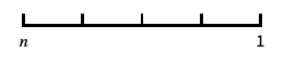
座標の向きを逆にする
全オプションのリスト
例題
すべて開く すべて閉じる例 (2)
data = Table[x y z, {z, -1, 1, 2 / 40.}, {y, -1, 1, 2 / 40.}, {x, -1, 1, 2 / 40.}];ListDensityPlot3D[data]data = Table[Sin[x]Cos[y]Sin[z], {z, -5, 5, 0.1}, {y, -5, 5, 0.1}, {x, -5, 5, 0.1}];ListDensityPlot3D[data, ColorFunction -> "TemperatureMap", PlotLegends -> Automatic]スコープ (16)
データ (7)
 値からなる規則的なデータについては,
 ,
 ,
 データは配列中の自身の位置を反映する:
data = Table[Sin[x]Cos[y]Sin[z], {z, 0, 2 Pi, 2Pi / 30}, {y, 0, 2Pi, 2Pi / 30}, {x, 0, 2Pi, 2Pi / 30}];ListDensityPlot3D[data]DataRangeを使って  ,
 ,
 の明示的なデータ範囲を与える:
ListDensityPlot3D[data, DataRange -> {{0, 2Pi}, {0, 2Pi}, {0, 2Pi}}]


data = Flatten[Table[{x, y, z, ChessboardDistance[{x, y, z}, {0, 0, 0}]}, {z, -1, 1, 2 / 9}, {y, -1, 1, 2 / 9}, {x, -1, 1, 2 / 9}], 2];ListDensityPlot3D[data]不規則データ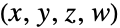 については,
 ,
 ,
 のデータ範囲はデータから推定される:
pts = RandomPoint[Cuboid[], 10 ^ 3];
data = Table[Append[p, Sqrt[p[[1]] ^ 2 + p[[2]] ^ 2 + p[[3]] ^ 2]], {p, pts}];ListDensityPlot3D[data]RegionFunctionを使ってより一般的にデータの包含を制約する:
data = Table[x y z, {z, -1, 1, 2 / 40.}, {y, -1, 1, 2 / 40.}, {x, -1, 1, 2 / 40.}];ListDensityPlot3D[data, RegionFunction -> Function[{x, y, z}, x ^ 2 + y ^ 2 + z ^ 2 ≤ 1], DataRange -> {{-1, 1}, {-1, 1}, {-1, 1}}]SparseArrayで与えられた値の配列について,密度をプロットする:
data = SparseArray[Flatten[Table[{i ^ 2, j ^ 2, k ^ 2} -> i j k, {i, 1, 4}, {j, 1, 4}, {k, 1, 4}]]];ListDensityPlot3D[data]QuantityArrayで与えられた値の配列について,密度をプロットする:
data = QuantityArray[Table[x y z, {z, -1, 1, .05}, {y, -1, 1, .05}, {x, -1, 1, .05}], "kg/m^3"];ListDensityPlot3D[data, AxesLabel -> Automatic, PlotLegends -> Automatic, TargetUnits -> {"Feet", "Feet", "Feet", "g/ft^3"}]ClipPlanesを使って1つあるいは複数の切り取り平面を指定する.この場合は を切り取る:
data = Table[Sin[x]Cos[y]Sin[z], {z, 0, 2 Pi, 2Pi / 30}, {y, 0, 2Pi, 2Pi / 30}, {x, 0, 2Pi, 2Pi / 30}];ListDensityPlot3D[data, ClipPlanes -> {{-1, 1, -1, 2}}, OpacityFunction -> None, DataRange -> {{0, 2Pi}, {0, 2Pi}, {0, 2Pi}}]表形式データ (1)
プレゼンテーション (8)
PlotThemeを使って全体的なスタイルを即座に得る:
data = Table[x y z, {z, -1, 1, .05}, {y, -1, 1, .05}, {x, -1, 1, .05}];Table[ListDensityPlot3D[data, PlotLabel -> t, PlotTheme -> t], {t, {"Minimal", "Scientific", "Marketing"}}]PlotLegendsを使ってさまざまな値についての色の棒を得る:
data = Table[x y z, {z, -1, 1, .05}, {y, -1, 1, .05}, {x, -1, 1, .05}];ListDensityPlot3D[data, PlotLegends -> Automatic]Axesで軸の表示を制御する:
data = Table[x y z, {z, -1, 1, .05}, {y, -1, 1, .05}, {x, -1, 1, .05}];Table[ListDensityPlot3D[data, PlotLabel -> a, Axes -> a], {a, {True, False, {True, False, True}}}]AxesLabelを使って軸に,PlotLabelを使ってプロット全体にラベルを付ける:
data = Table[x y z, {z, -1, 1, .05}, {y, -1, 1, .05}, {x, -1, 1, .05}];ListDensityPlot3D[data, Ticks -> None, AxesLabel -> {x, y, z}, PlotLabel -> x y z]ColorFunctionを使い,関数の値でプロットに彩色する:
data = Table[x y z, {z, -1, 1, .05}, {y, -1, 1, .05}, {x, -1, 1, .05}];Table[ListDensityPlot3D[data, PlotLabel -> c, ColorFunction -> c], {c, {Hue, "BlueGreenYellow"}}]カスタムの不透明性関数を使って各点の体積の不透明度を指定する:
data = Table[Sin[π x]Sin[π (y + z)], {z, -2, 2, 0.1}, {y, -2, 2, 0.1}, {x, -2, 2, 0.1}];ListDensityPlot3D[data, OpacityFunction -> (If[# < 0.7, 1, 0]&)]TargetUnitsは可視化で使う単位を指定する:
data = QuantityArray[Table[x y z, {z, -1, 1, .05}, {y, -1, 1, .05}, {x, -1, 1, .05}], "kg/m^3"];ListDensityPlot3D[data, AxesLabel -> Automatic, PlotLegends -> Automatic, TargetUnits -> {"Feet", "Feet", "Feet", "g/ft^3"}]x 方向にScalingFunctionsを使う:
ListDensityPlot3D[Table[Sin[π x]Sin[π (y + z)], {z, -2, 2, 0.05}, {y, -2, 2, 0.05}, {x, -2, 2, 0.05}], ScalingFunctions -> {"Log", None, None}]オプション (38)
BoxRatios (3)
data = Table[Sin[2π x]Sin[2π y]Sin[2π z], {z, -Pi, Pi, 0.1}, {y, -1, 1, 0.1}, {x, -1, 1, 0.1}];ListDensityPlot3D[data]BoxRatiosAutomaticを使って3D座標値の自然なスケールを示す:
data = Table[Sin[2π x]Sin[2π y]Sin[2π z], {z, -Pi, Pi, 0.1}, {y, -1, 1, 0.1}, {x, -1, 1, 0.1}];ListDensityPlot3D[data, BoxRatios -> Automatic]data = Table[Sin[2π x]Sin[2π y]Sin[2π z], {z, -Pi, Pi, 0.1}, {y, -1, 1, 0.1}, {x, -1, 1, 0.1}];ListDensityPlot3D[data, BoxRatios -> {5, 2, 3}]ClipPlanes (3)
ClipPlanesを使って切取り平面を指定する.この場合は 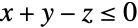 を切り取る:
data = Table[Sin[x + y + z] / 10, {z, 0, 10, .5}, {y, 0, 10, .5}, {x, 0, 10, .5}];ListDensityPlot3D[data, DataRange -> {{0, 10}, {0, 10}, {0, 10}}, OpacityFunction -> None, ClipPlanes -> {{1, 1, -1, 0}}]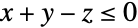
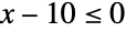
data = Table[Sin[x + y + z] / 10, {z, 0, 10, .5}, {y, 0, 10, .5}, {x, 0, 10, .5}];ListDensityPlot3D[data, OpacityFunction -> None, ClipPlanes -> {{1, 1, -1, 0}, {0, 1, 0, -4}}, DataRange -> {{0, 10}, {0, 10}, {0, 10}}]一般的なRegionFunctionと比較する:
data = Table[Sin[x + y + z] / 10, {z, 0, 10, .5}, {y, 0, 10, .5}, {x, 0, 10, .5}];ListDensityPlot3D[data, OpacityFunction -> None, RegionFunction -> Function[{x, y, z}, x + y - z ≤ 0], DataRange -> {{0, 10}, {0, 10}, {0, 10}}]ColorFunction (2)


data = Table[Sin[(i + j + k) / 20], {i, 0, 20}, {j, 0, 20}, {k, 0, 20}];ListDensityPlot3D[data, ColorFunction -> Hue]ColorDataからの色関数を使う:
data = Table[PDF[DirichletDistribution[{1, 2, 3, 4}], {x, y, z}], {z, 0, 1, 0.05}, {y, 0, 1, 0.05}, {x, 0, 1, 0.05}];Table[ListDensityPlot3D[data, ColorFunction -> cf, DataRange -> {{0, 1}, {0, 1}, {0, 1}}], {cf, {"AlpineColors", "Aquamarine", "ArmyColors", "AtlanticColors"}}]ColorFunctionScaling (2)
ColorFunctionのパラメータは0から1の間に通常にスケールされる:
ListDensityPlot3D[Table[x + y + z, {z, 0, 3, 0.2}, {y, 0, 3, 0.2}, {x, 0, 3, 0.2}], ColorFunction -> Hue]ColorFunctionScalingをFalseに設定することでスケールされていない座標を使う:
data = Table[x + y + z, {z, 0, 3, 0.2}, {y, 0, 3, 0.2}, {x, 0, 3, 0.2}];ListDensityPlot3D[data, ColorFunction -> Hue, ColorFunctionScaling -> False]DataRange (2)
data = Table[Exp[-(x ^ 2 + y ^ 2 + z ^ 2)], {z, -1, 1, 1 / 10}, {y, -1, 1, 1 / 20}, {x, -1, 1, 1 / 30}];ListDensityPlot3D[data, DataRange -> Automatic]data = Table[Exp[-(x ^ 2 + y ^ 2 + z ^ 2)], {z, -1, 1, 1 / 10}, {y, -1, 1, 1 / 20}, {x, -1, 1, 1 / 30}];ListDensityPlot3D[data, DataRange -> {{-1, 1}, {-1, 1}, {-1, 1}}]MaxPlotPoints (1)
OpacityFunction (5)
OpacityFunctionは,デフォルトでAutomaticである:
data = Table[x ^ 2 + y ^ 2 + z ^ 2, {z, -2, 2, 0.1}, {y, -2, 2, 0.1}, {x, -2, 2, 0.1}];ListDensityPlot3D[data]Noneを使って立体全体を不透明にする:
data = Table[Sin[π x]Sin[π (y + z)], {z, -2, 2, 0.1}, {y, -2, 2, 0.1}, {x, -2, 2, 0.1}];ListDensityPlot3D[data, OpacityFunction -> None]カスタムの不透明度関数を使って各点立体の不透明度を指定する:
data = Table[Sin[π x]Sin[π (y + z)], {z, -2, 2, 0.1}, {y, -2, 2, 0.1}, {x, -2, 2, 0.1}];ListDensityPlot3D[data, OpacityFunction -> (If[# < 0.4, 1, 0]&)]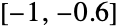

data = Table[Sin[π x]Sin[π y] Sin[π z], {z, -1, 1, 0.05}, {y, -1, 1, 0.05}, {x, -1, 1, 0.05}];ListDensityPlot3D[data, OpacityFunction -> Interval[{-1, -0.6}, {0.6, 1}], OpacityFunctionScaling -> False, PlotLegends -> Automatic, DataRange -> {{-1, 1}, {-1, 1}, {-1, 1}}]一定した不透明度Opacity[0.05]を使う:
data = Table[Sin[π x]Sin[π y] Sin[π z], {z, -1, 1, 0.05}, {y, -1, 1, 0.05}, {x, -1, 1, 0.05}];ListDensityPlot3D[data, OpacityFunction -> 0.05, PlotLegends -> Automatic, DataRange -> {{-1, 1}, {-1, 1}, {-1, 1}}]OpacityFunctionScaling (2)
data = Table[x y z, {z, -5, 5}, {y, -5, 5}, {x, -5, 5}];ListDensityPlot3D[data, OpacityFunction -> Function[f, If[f > 0, 1, 0]]]OpacityFunctionScalingをFalseに設定してスケールされていない密度の値を使う:
data = Table[x y z, {z, -5, 5}, {y, -5, 5}, {x, -5, 5}];ListDensityPlot3D[data, OpacityFunction -> Function[f, If[f > 0, 1, 0]], OpacityFunctionScaling -> False]PerformanceGoal (2)
data = Table[x y z, {z, -1, 1, .1}, {y, -1, 1, .1}, {x, -1, 1, .1}];Timing[ListDensityPlot3D[data, PerformanceGoal -> "Quality"]]data = Table[x y z, {z, -1, 1, .1}, {y, -1, 1, .1}, {x, -1, 1, .1}];Timing[ListDensityPlot3D[data, PerformanceGoal -> "Speed"]]PlotLegends (2)
data = Table[x y z, {x, -1, 1, 2 / 40.}, {y, -1, 1, 2 / 40.}, {z, -1, 1, 2 / 40.}];ListDensityPlot3D[data]PlotLegends->Automaticを使って凡例の付いたプロットを示す:
data = Table[x y z, {z, -1, 1, 2 / 40.}, {y, -1, 1, 2 / 40.}, {x, -1, 1, 2 / 40.}];ListDensityPlot3D[data, PlotLegends -> Automatic]PlotRange (3)
data = Table[Exp[-(x ^ 2 + y ^ 2 + z ^ 2)], {z, -1, 1, 1 / 20}, {y, -1, 1, 1 / 20}, {x, -1, 1, 1 / 20}];ListDensityPlot3D[data, DataRange -> {{-1, 1}, {-1, 1}, {-1, 1}}]data = Table[Exp[-(x ^ 2 + y ^ 2 + z ^ 2)], {z, -1, 1, 1 / 20}, {y, -1, 1, 1 / 20}, {x, -1, 1, 1 / 20}];ListDensityPlot3D[data, DataRange -> {{-1, 1}, {-1, 1}, {-1, 1}}, PlotRange -> {{-1, 0}, All, All}, BoxRatios -> Automatic]data = Table[Exp[-(x ^ 2 + y ^ 2 + z ^ 2)], {z, -1, 1, 0.05}, {y, -1, 1, 0.05}, {x, -1, 1, 0.05}];ListDensityPlot3D[data, PlotRange -> {All, All, All, {0, 0.2}}]ListDensityPlot3D[data, PlotRange -> {0, 0.2}]PlotTheme (3)
data = Table[x y z, {z, -1, 1, 2 / 40.}, {y, -1, 1, 2 / 40.}, {x, -1, 1, 2 / 40.}];ListDensityPlot3D[data, PlotTheme -> "Detailed"]data = Table[x y z, {z, -1, 1, 2 / 40.}, {y, -1, 1, 2 / 40.}, {x, -1, 1, 2 / 40.}];ListDensityPlot3D[data, PlotTheme -> "Detailed", FaceGrids -> None]data = Table[x y z, {z, -1, 1, 2 / 40.}, {y, -1, 1, 2 / 40.}, {x, -1, 1, 2 / 40.}];Table[ListDensityPlot3D[data, PlotLabel -> t, PlotTheme -> t, ImageSize -> 130], {t, {"Scientific", "Monochrome", "Minimal", "Web", "Working", "Classic", "Business", "Marketing", "Detailed"}}]RegionFunction (3)


data = Table[x y z, {z, -1, 1, 2 / 40.}, {y, -1, 1, 2 / 40.}, {x, -1, 1, 2 / 40.}];ListDensityPlot3D[data, RegionFunction -> Function[{x, y, z}, x ^ 2 + y ^ 2 + z ^ 2 ≤ 1], DataRange -> {{-1, 1}, {-1, 1}, {-1, 1}}]
data = Table[x ^ 2 + y ^ 2 - z ^ 2, {z, -2, 2, .2}, {y, -2, 2, .2}, {x, -2, 2, .2}];ListDensityPlot3D[data, RegionFunction -> Function[{x, y, z, f}, f < 2], DataRange -> {{-2, 2}, {-2, 2}, {-2, 2}}]data = Table[x ^ 2 + y ^ 2 - z ^ 2, {z, -2, 2, .2}, {y, -2, 2, .2}, {x, -2, 2, .2}];ListDensityPlot3D[data, RegionFunction -> Function[{x, y, z, f}, x < -1 || x > 1], DataRange -> {{-2, 2}, {-2, 2}, {-2, 2}}]ScalingFunctions (4)
デフォルトで,プロットではすべての方向に線形スケールが使われる:
ListDensityPlot3D[Table[Cos[x + y + z] / 10, {z, 0, 10, .25}, {y, 0, 10, .25}, {x, 0, 10, .25}]]
ListDensityPlot3D[Table[Cos[x + y + z] / 10, {z, 0, 10, .25}, {y, 0, 10, .25}, {x, 0, 10, .25}], ScalingFunctions -> {"Log", None, None}]ScalingFunctionsを使って  方向の座標の向きが逆になるようにスケールする:
ListDensityPlot3D[Table[Cos[x + y + z] / 10, {z, 0, 10, .25}, {y, 0, 10, .25}, {x, 0, 10, .25}], ScalingFunctions -> {None, None, "Reverse"}]ListDensityPlot3D[Table[Cos[x + y + z] / 10, {z, 0, 10, .25}, {y, 0, 10, .25}, {x, 0, 10, .25}], ScalingFunctions -> {None, None, {-Log[#]&, Exp[-#]&}}]TargetUnits (1)
data = QuantityArray[Table[Exp[-(x ^ 2 + y ^ 2 + z ^ 2)], {z, -2, 2, 0.1}, {y, -2, 2, 0.1}, {x, -2, 2, 0.1}], "Feet"];ListDensityPlot3D[data, TargetUnits -> {"Meters", "Meters", "Meters", "Meters"}, PlotLegends -> Automatic, AxesLabel -> Automatic]アプリケーション (13)
初等関数 (4)

data = Table[x, {z, -2, 2}, {y, -2, 2}, {x, -2, 2, 0.25}];ListDensityPlot3D[data]

{ListDensityPlot3D[Table[y, {z, -2, 2}, {y, -2, 2, 0.25}, {x, -2, 2}]],
	ListDensityPlot3D[Table[z, {z, -2, 2, 0.25}, {y, -2, 2}, {x, -2, 2}]]}

{ListDensityPlot3D[Table[x + y, {z, -2, 2}, {y, -2, 2, 0.25}, {x, -2, 2, 0.25}]],
	ListDensityPlot3D[Table[y + z, {z, -2, 2, 0.25}, {y, -2, 2, 0.25}, {x, -2, 2}]]}

{ListDensityPlot3D[Table[x + y + z, {z, -2, 2, 0.25}, {y, -2, 2, 0.25}, {x, -2, 2, 0.25}]],
	ListDensityPlot3D[Table[x - y + z, {x, -2, 2, 0.2}, {y, -2, 2, 0.2}, {z, -2, 2, 0.2}]]}

{ListDensityPlot3D[Table[x ^ 2 + y ^ 2, {z, -2, 2}, {y, -2, 2, 0.25}, {x, -2, 2, 0.25}]], ListDensityPlot3D[Table[y ^ 2 + z ^ 2, {z, -2, 2, 0.25}, {y, -2, 2, 0.25}, {x, -2, 2}]]}

{ListDensityPlot3D[Table[x ^ 2 + y ^ 2 + z ^ 2, {z, -2, 2, 0.2}, {y, -2, 2, 0.2}, {x, -2, 2, 0.2}]], ListDensityPlot3D[Table[x ^ 2 + y ^ 2 + 2z ^ 2, {z, -2, 2, 0.2}, {y, -2, 2, 0.2}, {x, -2, 2, 0.2}]]}
ListDensityPlot3D[Table[Sin[π x]Sin[π y]Sin[π z], {z, -2, 2, 0.1}, {y, -2, 2, 0.1}, {x, -2, 2, 0.1}]]

{ListDensityPlot3D[Table[Sin[π x]Sin[π (y + z)], {z, -2, 2, 0.1}, {y, -2, 2, 0.1}, {x, -2, 2, 0.1}]], ListDensityPlot3D[Table[Sin[π (x + y)]Sin[π z], {z, -2, 2, 0.1}, {y, -2, 2, 0.1}, {x, -2, 2, 0.1}]]}
ListDensityPlot3D[Table[Sin[π (x + y + z)], {z, -2, 2, 0.1}, {y, -2, 2, 0.1}, {x, -2, 2, 0.1}]]
f = Exp[-Norm[{x, y, z} - {-1, -1, -1}]^2] + Exp[-Norm[{x, y, z} - {1, 1, 1}]^2];ListDensityPlot3D[Table[f, {z, -2, 2, 0.2}, {y, -2, 2, 0.2}, {x, -2, 2, 0.2}]]
f = Sum[Exp[-2Norm[{x, y, z} - pi]^2], {pi, RandomPoint[Cuboid[{-1, -1, -1}, {1, 1, 1}], 10]}];ListDensityPlot3D[Table[f, {x, -2, 2, 0.2}, {y, -2, 2, 0.2}, {z, -2, 2, 0.2}]]シミュレーションデータ (6)
𝒟 = ProductDistribution[{LogNormalDistribution[0, 1], 3}];
f = PDF[𝒟, {x, y, z}]ListDensityPlot3D[Table[f, {z, 0, 3, .1}, {y, 0, 3, .1}, {x, 0, 3, .1}], DataRange -> {{0, 3}, {0, 3}, {0, 3}}]data = Last@HistogramList[RandomVariate[𝒟, 10 ^ 6], {0, 3, 0.1}];ListDensityPlot3D[data]walk = Accumulate[RandomInteger[{-1, 1}, {10 ^ 5, 3}]];Graphics3D[Line[walk], BoxRatios -> 1, Axes -> True]data = Last@HistogramList[walk];ListDensityPlot3D[data, PlotLegends -> Automatic, DataRange -> CoordinateBounds[walk]]data = CellularAutomaton[{2274, {2, 1}, {1, 1, 1}}, {{{{1}}}, 0}, {20, {{10}}}];ListDensityPlot3D[data]data = Last@SubstitutionSystem[{1 -> 1 - CrossMatrix[{1, 1, 1}], 0 -> ConstantArray[0, {3, 3, 3}]}, {{{1}}}, 3];ListDensityPlot3D[data, OpacityFunction -> (#&), ColorFunction -> GrayLevel]data = Last@SubstitutionSystem[{1 -> ArrayReshape[IntegerDigits[45115427, 2, 27], {3, 3, 3}], 0 -> ConstantArray[0, {3, 3, 3}]}, {{{1}}}, 3];ListDensityPlot3D[data]配列中の半径1の近傍を平均することで,ランダムな値の二次元配列の離散拡散モデルのシミュレーションを行う:
g[d_] := ArrayFilter[Total[#, 2] / 9&, d, 1];ListDensityPlot3D[NestList[g, RandomReal[1, {40, 40}], 40], PlotLegends -> Automatic, AxesLabel -> {None, None, "time"}]データパターン (3)
data = Arg[Fourier[Table[1 / LCM[i, j, k], {i, 64}, {j, 64}, {k, 64}]]];ListDensityPlot3D[data]positions = ProteinData["RAB21", "AtomPositions"];data = Last@HistogramList[positions];ListDensityPlot3D[data, PlotLegends -> Automatic]ProteinData["RAB21", "MoleculePlot"]data = ExampleData[{"TestImage3D", "MRbrain"}, "GrayLevels"];ListDensityPlot3D[data, BoxRatios -> Automatic]Image3Dと同じ方向にするためには,オプションDataReversedを使う:
data = ImageData[ExampleData[{"TestImage3D", "MRbrain"}, "Image3D"], DataReversed -> True];ListDensityPlot3D[data, BoxRatios -> Automatic]特性と関係 (6)
ListSliceDensityPlot3Dをスライス平面上の密度点に使う:
data = Table[x y z, {z, -2, 2, .1}, {y, -2, 2, .1}, {x, -2, 2, .1}];{ListSliceDensityPlot3D[data, "BackPlanes"], ListDensityPlot3D[data]}ListDensityPlotを2Dの密度プロットに使う:
data = Table[x ^ 2 + y ^ 2, {z, -1, 1, .1}, {y, -1, 1, .1}, {x, -1, 1, .1}];{ListDensityPlot[First[data]], ListDensityPlot3D[data, OpacityFunction -> None]}DensityPlot3Dを関数に使う:
data = Table[x y z, {z, -1, 1, 0.05}, {y, -1, 1, 0.05}, {x, -1, 1, 0.05}];{DensityPlot3D[x y z, {x, -2, 2}, {y, -2, 2}, {z, -2, 2}], ListDensityPlot3D[data]}ListSliceContourPlot3Dをスライド表面上の等高線に使う:
data = Table[x ^ 2 + y ^ 2 + z ^ 2, {z, -2, 2, .1}, {y, -2, 2, .1}, {x, -2, 2, .1}];{ListSliceContourPlot3D[data], ListDensityPlot3D[data]}ListContourPlot3Dを一定値の表面に使う:
data = Table[x ^ 2 + y ^ 2 + z ^ 2, {z, -2, 2, .1}, {y, -2, 2, .1}, {x, -2, 2, .1}];{ListContourPlot3D[data], ListDensityPlot3D[data]}ArrayPlot3Dを離散データに使う:
data = Table[GCD[x, y, z] - 1, {z, -5, 5}, {y, -5, 5}, {x, -5, 5}];{ArrayPlot3D[data], ListDensityPlot3D[data]}テキスト
Wolfram Research (2015), ListDensityPlot3D, Wolfram言語関数, https://reference.wolfram.com/language/ref/ListDensityPlot3D.html (2025年に更新).
CMS
Wolfram Language. 2015. "ListDensityPlot3D." Wolfram Language & System Documentation Center. Wolfram Research. Last Modified 2025. https://reference.wolfram.com/language/ref/ListDensityPlot3D.html.
APA
Wolfram Language. (2015). ListDensityPlot3D. Wolfram Language & System Documentation Center. Retrieved from https://reference.wolfram.com/language/ref/ListDensityPlot3D.html