


ListSliceContourPlot3D
ListSliceContourPlot3D[farr,surf]
generates a contour plot of the three-dimensional farr of values sliced to the surface surf.
ListSliceContourPlot3D[{{x1,y1,z1,f1},{x2,y2,z2,f2},…},surf]
generates a slice contour plot for the values fi at points {xi,yi,zi}.
ListSliceContourPlot3D[…,{surf1,surf2,…}]
generates slice contour plots over several slices surf1, surf2, ….
Details and Options
- ListSliceContourPlot3D gives smooth contours on surfaces in a volume.
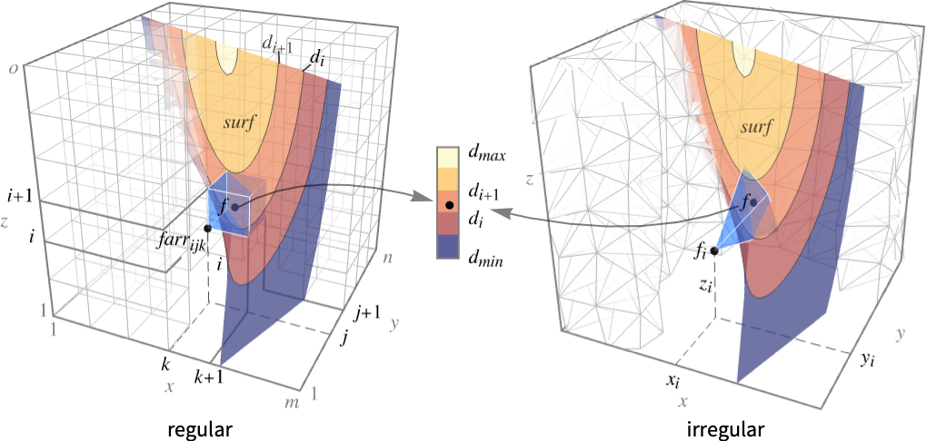
- ListSliceContourPlot3D constructs contour curves on the surface surf corresponding to the level sets where the interpolated function
 has constant values d1, d2, etc. By default, the regions between the curves are shaded to more easily identify regions whose values are between di and di+1.
 - For regular data, the function
 has value farr[[i,j,k]] at
  .
. - For irregular data,
 has value fi at
  .
. - It visualizes the surfaces
 where the region
  is the Cartesian product
  for regular data and the convex hull of {{x1,y1,z1},…,{xn,yn,zn}} for irregular data.
 - ListSliceContourPlot3D[Tabular[…]cspec] extracts and plots values from the tabular object using the column specification cspec.
- The following forms of column specifications cspec are allowed for plotting tabular data:
-
{colx,coly,colz,colf} plot column f against columns x, y and z - The following basic slice surfaces surfi can be given:
-
Automatic automatically determine slice surfaces 
"CenterPlanes" coordinate planes through the center 
"BackPlanes" coordinate planes at the back of the plot 
"XStackedPlanes" coordinate planes stacked along  axis
axis
"YStackedPlanes" coordinate planes stacked along  axis
axis
"ZStackedPlanes" coordinate planes stacked along  axis
axis
"DiagonalStackedPlanes" planes stacked diagonally 
"CenterSphere" a sphere in the center 
"CenterCutSphere" a sphere with a cutout wedge 
"CenterCutBox" a box with a cutout octant - ListSliceContourPlot3D[data] is equivalent to ListSliceContourPlot3D[data,Automatic].
- The following parametrizations can be used for basic slice surfaces:
-
{"XStackedPlanes",n}, generate n equally spaced planes {"XStackedPlanes",{x1,x2,…}} generate planes for x=xi {"CenterCutSphere",ϕopen} cut angle ϕopen facing the view point {"CenterCutSphere",ϕopen,ϕcenter} cut angle ϕopen with center angle ϕcenter in  plane
plane - "YStackedPlanes", "ZStackedPlanes" follow the specifications for "XStackedPlanes", with additional features shown in the scope examples.
- The following general slice surfaces surfi can be used:
-
surfaceregion a two-dimensional region in 3D, e.g. Hyperplane volumeregion a three-dimensional region in 3D where surfi is taken as the boundary surface, e.g. Cuboid - The following wrappers can be used for slice surfaces surfi:
-
Annotation[surf,label] provide an annotation Button[surf,action] define an action to execute when the surface is clicked EventHandler[surf,…] define a general event handler for the surface Hyperlink[surf,uri] make the surface act as a hyperlink PopupWindow[surf,cont] attach a popup window to the surface StatusArea[surf,label] display in status area when the surface is moused over Tooltip[surf,label] attach an arbitrary tooltip to the surface - ListSliceContourPlot3D has the same options as Graphics3D, with the following additions and changes: [List of all options]
-
Axes True whether to draw axes BoundaryStyle Automatic how to style surface boundaries BoxRatios {1,1,1} bounding 3D box ratios ClippingStyle None how to draw values clipped by PlotRange ColorFunction Automatic how to color the plot ColorFunctionScaling True whether to scale the arguments to ColorFunction Contours Automatic how many or what contours to show on each surface ContourShading Automatic how to shade regions between contours ContourStyle Automatic the style for contour lines DataRange Automatic the range of x, y, and z values to assume for data PerformanceGoal $PerformanceGoal aspects of performance to optimize PlotLegends None legends for color gradients PlotPoints Automatic approximate number of samples for the slice surfaces surfi in each direction PlotRange {Full,Full,Full,Automatic} range of f or other values to include PlotTheme $PlotTheme overall theme for the plot RegionFunction (True&) how to determine whether a point should be included ScalingFunctions None how to scale individual coordinates TargetUnits Automatic desired units to use - ColorFunction is by default supplied with the scaled value of f.
- RegionFunction is by default supplied with x, y, z, and f.
- For a farr of dimension {r,s,t}, the setting DataRangeAutomatic is equivalent to DataRange{{1,r},{1,s},{1,t}}.
- Possible settings for ScalingFunctions include:
-
sf scale the fcontour values {sx,sy,sz} scale x, y and z axes {sx,sy,sz,sf} scale x, y and z axes and fcontour values - Common built-in scaling functions s include:
-
"Log" 
log scale with automatic tick labeling "Log10" 
base-10 log scale with powers of 10 for ticks "SignedLog" 
log-like scale that includes 0 and negative numbers "Reverse" 
reverse the coordinate direction
List of all options
Examples
open all close allBasic Examples (2)
Plot the contours of an array of values over a set of surfaces:
data = Table[Sqrt[x ^ 2 + y ^ 2 + z ^ 2], {z, 0, 3, 0.1}, {y, 0, 3, 0.1}, {x, 0, 3, 0.1}];ListSliceContourPlot3D[data, "CenterPlanes"]Plot the contours over the surface ![]() :
:
data = Table[Exp[-(x ^ 2 + y ^ 2 + z ^ 2)], {z, -2, 2, 0.2}, {y, -2, 2, 0.2}, {x, -2, 2, 0.2}];ListSliceContourPlot3D[data, ImplicitRegion[x ^ 3 + y ^ 2 - z ^ 2 == 0, {x, y, z}], DataRange -> {{-2, 2}, {-2, 2}, {-2, 2}}]Scope (29)
Surfaces (9)
Generate a contour plot over standard slice surfaces:
data = Table[x + y + z, {z, -1, 1, 0.2}, {y, -1, 1, 0.2}, {x, -1, 1, 0.2}];Table[ListSliceContourPlot3D[data, sl, PlotLabel -> sl], {sl, {"CenterPlanes", "BackPlanes", "ZStackedPlanes"}}]Standard axis-aligned stacked slice surfaces:
data = Table[Sin[x] + y ^ 2 - z ^ 3, {z, -1, 1, 0.2}, {y, -1, 1, 0.2}, {x, -1, 1, 0.2}];Table[ListSliceContourPlot3D[data, sl, PlotLabel -> sl], {sl, {"XStackedPlanes", "YStackedPlanes", "ZStackedPlanes"}}]data = Table[Sin[x] + y ^ 2 - z ^ 3, {z, -1, 1, 0.2}, {y, -1, 1, 0.2}, {x, -1, 1, 0.2}];Table[ListSliceContourPlot3D[data, sl, PlotLabel -> sl], {sl, {"CenterSphere", "CenterCutSphere", "CenterCutBox"}}]Plot the contours over any surface region:
data = Table[x + y + z, {z, -1, 1}, {y, -1, 1}, {x, -1, 1}];ListSliceContourPlot3D[data, HalfPlane[{{0, 0, 0}, {1, 0, 0}}, {0, 1, 1}]]Plotting over a volume primitive is equivalent to plotting over RegionBoundary[reg]:
data = Table[x + y + z, {z, -1, 1}, {y, -1, 1}, {x, -1, 1}];ListSliceContourPlot3D[data, Cylinder[], DataRange -> {{-1, 1}, {-1, 1}, {-1, 1}}]Plot the contours over the surface ![]() :
:
data = Table[Sin[x y z], {z, -2, 2, 0.2}, {y, -2, 2, 0.2}, {x, -2, 2, 0.2}];ListSliceContourPlot3D[data, ImplicitRegion[x ^ 3 + y ^ 2 - z ^ 2 == 0, {x, y, z}], DataRange -> {{-2, 2}, {-2, 2}, {-2, 2}}]Plot the contours over multiple surfaces:
data = Table[Sin[x y z], {z, -2, 2, 0.2}, {y, -2, 2, 0.2}, {x, -2, 2, 0.2}];ListSliceContourPlot3D[data, {Cylinder[], "BackPlanes"}, Contours -> 3, DataRange -> {{-2, 2}, {-2, 2}, {-2, 2}}]Specify the number of stacked planes:
data = Table[x + y + z, {z, -2, 2}, {y, -2, 2}, {x, -2, 2}];ListSliceContourPlot3D[data, {"XStackedPlanes", 7}]Specify the cutting angle for a center-cut sphere slice:
data = Table[Sin[x y z], {z, -2, 2}, {y, -2, 2}, {x, -2, 2}];ListSliceContourPlot3D[data, {"CenterCutSphere", 2Pi / 3}]Data (8)
For regular data consisting of ![]() values, the
values, the ![]() ,
, ![]() , and
, and ![]() data reflects its positions in the array:
data reflects its positions in the array:
data = Table[Sqrt[x ^ 2 + y ^ 2 + z ^ 2], {z, 0, 3, 0.1}, {y, 0, 3, 0.1}, {x, 0, 3, 0.1}];ListSliceContourPlot3D[data, "CenterPlanes"]Provide explicit ![]() ,
, ![]() , and
, and ![]() data ranges by using DataRange:
data ranges by using DataRange:
ListSliceContourPlot3D[data, "CenterPlanes", DataRange -> {{0, 3}, {0, 3}, {0, 3}}]Plot interpolated contours from irregular data consisting of (![]() ,
, ![]() ,
, ![]() ,
, ![]() ) tuples:
) tuples:
pts = RandomPoint[Cuboid[], 10 ^ 3];
data = Table[Append[p, p[[1]] + p[[2]] + p[[3]]], {p, pts}];ListSliceContourPlot3D[data, "CenterPlanes"]Show the points where the data values are provided:
Show[%, Graphics3D[{AbsolutePointSize[2], Red, Point[pts]}]]Plot the contours for an array of values given by SparseArray:
data = SparseArray@Table[Sqrt[x ^ 2 + y ^ 2 + z ^ 2], {z, 0, 3, 0.1}, {y, 0, 3, 0.1}, {x, 0, 3, 0.1}]ListSliceContourPlot3D[data]Plot the density for an array of values given by QuantityArray:
data = QuantityArray[Table[x ^ 2 + y ^ 2 + z ^ 2, {z, -2, 2, 0.5}, {y, -2, 2, 0.5}, {x, -2, 2, 0.5}], "kg/m^3"];ListSliceContourPlot3D[data, "BackPlanes", AxesLabel -> Automatic, PlotLegends -> Automatic, TargetUnits -> {"Meters", "Meters", "Meters", "g/ft^3"}]Use Contours to specify the number of contours:
data = Table[x + y + z, {z, -2, 2}, {y, -2, 2}, {x, -2, 2}];ListSliceContourPlot3D[data, "BackPlanes", Contours -> 5]Or the list of function values ![]() to put contours:
to put contours:
ListSliceContourPlot3D[data, "BackPlanes", Contours -> {-1, 0, 1}]Use PlotPoints to control sampling of surfaces:
data = Table[x ^ 2 + y ^ 2 + z ^ 2, {z, -1, 1}, {y, -1, 1}, {x, -1, 1}];Table[ListSliceContourPlot3D[data, "CenterPlanes", PlotLabel -> pp, Axes -> False, Boxed -> False, PlotPoints -> pp], {pp, {3, 6, 9}}]Areas where the function becomes nonreal are excluded:
data = Table[Sqrt[x y z], {z, -1, 1, 0.1}, {y, -1, 1, 0.1}, {x, -1, 1, 0.1}];ListSliceContourPlot3D[data, "CenterSphere", DataRange -> {{-1, 1}, {-1, 1}, {-1, 1}}]Use RegionFunction to expose obscured slices:
data = Table[x ^ 2 + y ^ 2 + z ^ 2, {z, -2, 2}, {y, -2, 2}, {x, -2, 2}];ListSliceContourPlot3D[data, "ZStackedPlanes", RegionFunction -> Function[{x, y, z}, x < 0 || y > 0], DataRange -> {{-2, 2}, {-2, 2}, {-2, 2}}]Tabular Data (1)
tabular = Tabular[IconizedObject[«data»], {"f", "x", "y", "z"}]Plot tabular data in which each column represents data in the form {x,y,z,f}:
ListSliceContourPlot3D[tabular -> {"x", "y", "z", "f"}]Include a legend for the plot:
ListSliceContourPlot3D[tabular -> {"x", "y", "z", "f"}, PlotLegends -> Automatic]Presentation (11)
Use PlotTheme to immediately get overall styling:
data = Table[x ^ 2 + y ^ 2 + z ^ 2, {z, -1, 1}, {y, -1, 1}, {x, -1, 1}];Table[ListSliceContourPlot3D[data, "CenterPlanes", PlotLabel -> t, PlotTheme -> t], {t, {"Minimal", "Scientific", "Marketing"}}]Use PlotLegends to get a color bar for the different values:
data = Table[x y z, {z, -1, 1}, {y, -1, 1}, {x, -1, 1}];ListSliceContourPlot3D[data, "BackPlanes", PlotLegends -> Automatic]Control the display of axes with Axes:
data = Table[x + y + z, {z, -1, 1}, {y, -1, 1}, {x, -1, 1}];Table[ListSliceContourPlot3D[data, "CenterPlanes", PlotLabel -> a, Axes -> a], {a, {True, False, {True, False, True}}}]Label axes using AxesLabel and the whole plot using PlotLabel:
data = Table[x ^ 2 + y ^ 2 + z ^ 2, {z, -2, 2}, {y, -2, 2}, {x, -2, 2}];ListSliceContourPlot3D[data, "CenterPlanes", Ticks -> None, AxesLabel -> {x, y, z}, PlotLabel -> x ^ 2 + y ^ 2 + z ^ 2]Color the plot by the data values with ColorFunction:
data = Table[x y z, {z, -1, 1}, {y, -1, 1}, {x, -1, 1}];Table[ListSliceContourPlot3D[data, "ZStackedPlanes", PlotLabel -> c, ColorFunction -> c], {c, {Hue, "BlueGreenYellow"}}]Style regions between contours with ContourShading:
data = Table[Exp[-(x ^ 2 + y ^ 2 + z ^ 2)], {z, -1, 1}, {y, -1, 1}, {x, -1, 1}];ListSliceContourPlot3D[data, "CenterPlanes", Contours -> 9, BoundaryStyle -> None, ContourShading -> {Orange, None, Blue}]Use ContourStyle to style the contour lines:
data = Table[x ^ 4 + y ^ 4 + z ^ 4 - x ^ 2 - y ^ 2 - z ^ 2, {z, -1, 1, 0.2}, {y, -1, 1, 0.2}, {x, -1, 1, 0.2}];ListSliceContourPlot3D[data, "CenterPlanes", ContourStyle -> Dotted]Style the slice surface boundaries with BoundaryStyle:
data = Table[Exp[-(x ^ 2 + y ^ 2 + z ^ 2)], {z, -2, 2, 0.5}, {y, -2, 2, 0.5}, {x, -2, 2, 0.5}];ListSliceContourPlot3D[data, "CenterPlanes", BoundaryStyle -> Gray]TargetUnits specifies which units to use in the visualization:
data = QuantityArray[Table[x ^ 2 + y ^ 2 + z ^ 2, {z, -2, 2, 0.5}, {y, -2, 2, 0.5}, {x, -2, 2, 0.5}], "kg/m^3"];ListSliceContourPlot3D[data, "BackPlanes", AxesLabel -> Automatic, PlotLegends -> Automatic, TargetUnits -> {"Feet", "Feet", "Feet", "g/ft^3"}]Create a plot with a log-scaled ![]() axis:
axis:
ListSliceContourPlot3D[IconizedObject[«data»], ScalingFunctions -> {"Log", None, None}]Reverse the coordinate direction in the ![]() direction:
direction:
ListSliceContourPlot3D[IconizedObject[«data»], ScalingFunctions -> {None, None, "Reverse"}]Options (68)
Axes (3)
ListSliceContourPlot3D[IconizedObject[«data»], "CenterPlanes"]Use AxesFalse to turn off the axes:
ListSliceContourPlot3D[IconizedObject[«data»], "CenterPlanes", Axes -> False]Turn on each axis individually:
{ListSliceContourPlot3D[IconizedObject[«data»], "CenterPlanes", Axes -> {False, False, True}], ListSliceContourPlot3D[IconizedObject[«data»], "CenterPlanes", Axes -> {False, True, False}], ListSliceContourPlot3D[IconizedObject[«data»], "CenterPlanes", Axes -> {True, False, False}]}AxesLabel (3)
No axes labels are drawn by default:
ListSliceContourPlot3D[IconizedObject[«data»], "CenterPlanes"]ListSliceContourPlot3D[IconizedObject[«data»], "CenterPlanes", AxesLabel -> z]ListSliceContourPlot3D[IconizedObject[«data»], "CenterPlanes", AxesLabel -> {"width", "depth", "height"}]AxesOrigin (2)
AxesStyle (4)
Change the style for the axes:
ListSliceContourPlot3D[IconizedObject[«data»], "CenterPlanes", AxesStyle -> Red]Specify the style of each axis:
ListSliceContourPlot3D[IconizedObject[«data»], "CenterPlanes", AxesStyle -> {{Thick, Brown}, {Thick, Blue}, {Thick, Green}}]Use different styles for the ticks and the axes:
ListSliceContourPlot3D[IconizedObject[«data»], "CenterPlanes", AxesStyle -> Green, TicksStyle -> StandardBlue]Use different styles for the labels and the axes:
ListSliceContourPlot3D[IconizedObject[«data»], "CenterPlanes", AxesStyle -> Green, LabelStyle -> StandardBlue]BoundaryStyle (1)
Style the slice surface boundaries with BoundaryStyle:
data = Table[-(x ^ 2 + y ^ 2 + z ^ 2), {z, -1, 1}, {y, -1, 1}, {x, -1, 1}];ListSliceContourPlot3D[data, "CenterPlanes", BoundaryStyle -> Gray]BoxRatios (3)
By default, the edges of the bounding box have the same length:
data = Table[x y z, {z, -1, 2, 0.5}, {y, 0, 1, 0.5}, {x, 0, 1, 0.5}];ListSliceContourPlot3D[data, "CenterSphere"]Use BoxRatios->Automatic to show the natural scale of the 3D coordinate values:
data = Table[x y z, {z, -1, 2, 0.5}, {y, 0, 1, 0.5}, {x, 0, 1, 0.5}];ListSliceContourPlot3D[data, "CenterSphere", BoxRatios -> Automatic]Use custom length ratios for each side of the bounding box:
data = Table[x y z, {z, -1, 2, 0.5}, {y, 0, 1, 0.5}, {x, 0, 1, 0.5}];ListSliceContourPlot3D[data, "CenterSphere", BoxRatios -> {1, 3, 2}]ClippingStyle (2)
data = Table[Exp[-(x ^ 2 + y ^ 2 + z ^ 2)], {z, -2, 2, 0.2}, {y, -2, 2, 0.2}, {x, -2, 2, 0.2}];ListSliceContourPlot3D[data, "CenterPlanes", PlotRange -> {0.09, 0.72}, ClippingStyle -> {Red, Blue}]Remove clipped regions with None:
data = Table[Exp[-(x ^ 2 + y ^ 2 + z ^ 2)], {z, -2, 2, 0.2}, {y, -2, 2, 0.2}, {x, -2, 2, 0.2}];ListSliceContourPlot3D[data, "CenterPlanes", PlotRange -> {0.09, 0.72}, ClippingStyle -> None]ColorFunction (3)
Color the contours according to the ![]() values:
values:
data = Table[x + y + z, {z, -1, 2, 0.5}, {y, 0, 1, 0.5}, {x, 0, 1, 0.5}];ListSliceContourPlot3D[data, "XStackedPlanes", ColorFunction -> Hue]Use a named color gradient from ColorData:
data = Table[x ^ 2 + y ^ 2 + z ^ 2, {z, -1, 2, 0.5}, {y, 0, 1, 0.5}, {x, 0, 1, 0.5}];ListSliceContourPlot3D[data, "XStackedPlanes", ColorFunction -> "IslandColors"]data = Table[Sin[2 x y z], {z, -2, 2, 0.1}, {y, -2, 2, 0.1}, {x, -2, 2, 0.1}];ListSliceContourPlot3D[data, "ZStackedPlanes", ColorFunction -> Function[f, If[f < 0, Red, Green]], ColorFunctionScaling -> False, Contours -> 3]ColorFunctionScaling (2)
By default, scaled values are used:
data = Table[x y z, {z, -2, 2}, {y, -2, 2}, {x, -2, 2}];ListSliceContourPlot3D[data, "BackPlanes", ColorFunction -> Hue]Use ColorFunctionScaling->False to get unscaled values:
data = Table[Sin[2 x y z], {z, -2, 2, 0.1}, {y, -2, 2, 0.1}, {x, -2, 2, 0.1}];ListSliceContourPlot3D[data, "BackPlanes", ColorFunction -> (If[# < 0, Red, Green]&), ColorFunctionScaling -> False, Contours -> 4, PlotPoints -> 50]Contours (4)
Use automatic contour selection:
data = Table[x ^ 3 + y ^ 2 - z ^ 2, {z, -2, 2}, {y, -2, 2}, {x, -2, 2}];ListSliceContourPlot3D[data, "BackPlanes", Contours -> Automatic]Use 5 equally spaced contours:
data = Table[x ^ 3 + y ^ 2 - z ^ 2, {z, -2, 2}, {y, -2, 2}, {x, -2, 2}];ListSliceContourPlot3D[data, "BackPlanes", Contours -> 5]Specify an explicit set of contours:
data = Table[x ^ 3 + y ^ 2 - z ^ 2, {z, -2, 2}, {y, -2, 2}, {x, -2, 2}];ListSliceContourPlot3D[data, "BackPlanes", Contours -> {-1, 1}]Use specific contours with specific styles:
data = Table[x ^ 3 + y ^ 2 - z ^ 2, {z, -2, 2}, {y, -2, 2}, {x, -2, 2}];ListSliceContourPlot3D[data, "BackPlanes", Contours -> {{-1, Red}, {1, Green}}]ContourStyle (1)
ContourShading (4)
ContourShadingAutomatic computes contour region shading from the ColorFunction:
data = Table[Exp[-(x ^ 2 + y ^ 2 + z ^ 2)], {z, -1, 1}, {y, -1, 1}, {x, -1, 1}];ListSliceContourPlot3D[data, "CenterPlanes", Contours -> 9, BoundaryStyle -> None, ContourShading -> Automatic, ColorFunction -> "BrightBands"]Cyclically repeat shading styles:
data = Table[Exp[-(x ^ 2 + y ^ 2 + z ^ 2)], {z, -1, 1}, {y, -1, 1}, {x, -1, 1}];ListSliceContourPlot3D[data, "CenterPlanes", Contours -> 9, BoundaryStyle -> None, ContourShading -> {Orange, Blue}]Leave every third contour region empty, starting from the second:
data = Table[Exp[-(x ^ 2 + y ^ 2 + z ^ 2)], {z, -1, 1}, {y, -1, 1}, {x, -1, 1}];ListSliceContourPlot3D[data, "CenterPlanes", Contours -> 9, BoundaryStyle -> None, ContourShading -> {Orange, None, Blue}]Leave the regions between contours blank:
data = Table[Exp[-(x ^ 2 + y ^ 2 + z ^ 2)], {z, -1, 1}, {y, -1, 1}, {x, -1, 1}];ListSliceContourPlot3D[data, "CenterPlanes", Contours -> 9, BoundaryStyle -> None, ContourShading -> None]DataRange (2)
By default, the data range is taken to be the dimension of the array:
data = Table[-(x ^ 2 + y ^ 2 + z ^ 2), {z, -2, 2}, {y, -2, 2}, {x, -2, 2}];ListSliceContourPlot3D[data, "XStackedPlanes"]Explicitly specify the data range:
data = Table[-(x ^ 2 + y ^ 2 + z ^ 2), {z, -2, 2}, {y, -2, 2}, {x, -2, 2}];ListSliceContourPlot3D[data, "XStackedPlanes", DataRange -> {{-2, 2}, {-2, 2}, {-2, 2}}]ImageSize (7)
Use named sizes such as Tiny, Small, Medium and Large:
{ListSliceContourPlot3D[Table[Exp[-(x ^ 2 + y ^ 2 + z ^ 2)], {z, -2, 2, 0.5}, {y, -2, 2, 0.5}, {x, -2, 2, 0.5}], "CenterPlanes", ImageSize -> Tiny], ListSliceContourPlot3D[Table[Exp[-(x ^ 2 + y ^ 2 + z ^ 2)], {z, -2, 2, 0.5}, {y, -2, 2, 0.5}, {x, -2, 2, 0.5}], "CenterPlanes", ImageSize -> Small]}Specify the width of the plot:
{ListSliceContourPlot3D[Table[Exp[-(x ^ 2 + y ^ 2 + z ^ 2)], {z, -2, 2, 0.5}, {y, -2, 2, 0.5}, {x, -2, 2, 0.5}], "CenterPlanes", ImageSize -> 150], ListSliceContourPlot3D[Table[Exp[-(x ^ 2 + y ^ 2 + z ^ 2)], {z, -2, 2, 0.5}, {y, -2, 2, 0.5}, {x, -2, 2, 0.5}], "CenterPlanes", AspectRatio -> 1.5, ImageSize -> 150]}Specify the height of the plot:
{ListSliceContourPlot3D[Table[Exp[-(x ^ 2 + y ^ 2 + z ^ 2)], {z, -2, 2, 0.5}, {y, -2, 2, 0.5}, {x, -2, 2, 0.5}], "CenterPlanes", ImageSize -> {Automatic, 150}], ListSliceContourPlot3D[Table[Exp[-(x ^ 2 + y ^ 2 + z ^ 2)], {z, -2, 2, 0.5}, {y, -2, 2, 0.5}, {x, -2, 2, 0.5}], "CenterPlanes", AspectRatio -> 2, ImageSize -> {Automatic, 150}]}Allow the width and height to be up to a certain size:
{ListSliceContourPlot3D[Table[Exp[-(x ^ 2 + y ^ 2 + z ^ 2)], {z, -2, 2, 0.5}, {y, -2, 2, 0.5}, {x, -2, 2, 0.5}], "CenterPlanes", ImageSize -> UpTo[200]], ListSliceContourPlot3D[Table[Exp[-(x ^ 2 + y ^ 2 + z ^ 2)], {z, -2, 2, 0.5}, {y, -2, 2, 0.5}, {x, -2, 2, 0.5}], "CenterPlanes", AspectRatio -> 2, ImageSize -> UpTo[200]]}Specify the width and height for a graphic, padding with space if necessary:
ListSliceContourPlot3D[Table[Exp[-(x ^ 2 + y ^ 2 + z ^ 2)], {z, -2, 2, 0.5}, {y, -2, 2, 0.5}, {x, -2, 2, 0.5}], "CenterPlanes", ImageSize -> {200, 200}, Background -> Lighter@Orange]Setting AspectRatioFull will fill the available space:
ListSliceContourPlot3D[Table[Exp[-(x ^ 2 + y ^ 2 + z ^ 2)], {z, -2, 2, 0.5}, {y, -2, 2, 0.5}, {x, -2, 2, 0.5}], "CenterPlanes", AspectRatio -> Full, ImageSize -> {200, 200}, Background -> Lighter@Orange]Use maximum sizes for the width and height:
{ListSliceContourPlot3D[Table[Exp[-(x ^ 2 + y ^ 2 + z ^ 2)], {z, -2, 2, 0.5}, {y, -2, 2, 0.5}, {x, -2, 2, 0.5}], "CenterPlanes", ImageSize -> {UpTo[150], UpTo[150]}], ListSliceContourPlot3D[Table[Exp[-(x ^ 2 + y ^ 2 + z ^ 2)], {z, -2, 2, 0.5}, {y, -2, 2, 0.5}, {x, -2, 2, 0.5}], "CenterPlanes", AspectRatio -> 2, ImageSize -> {UpTo[150], UpTo[150]}]}Use ImageSizeFull to fill the available space in an object:
Framed[Pane[ListSliceContourPlot3D[Table[Exp[-(x ^ 2 + y ^ 2 + z ^ 2)], {z, -2, 2, 0.5}, {y, -2, 2, 0.5}, {x, -2, 2, 0.5}], "CenterPlanes", ImageSize -> Full, Background -> Lighter@Orange], {200, 200}]]Specify the image size as a fraction of the available space:
Framed[Pane[ListSliceContourPlot3D[Table[Exp[-(x ^ 2 + y ^ 2 + z ^ 2)], {z, -2, 2, 0.5}, {y, -2, 2, 0.5}, {x, -2, 2, 0.5}], "CenterPlanes", AspectRatio -> Full, ImageSize -> {Scaled[0.5], Scaled[0.5]}, Background -> Lighter@Orange], {200, 200}]]PerformanceGoal (2)
Generate a higher-quality plot:
data = Table[-(x ^ 2 + y ^ 2 + z ^ 2), {z, -2, 2, 0.5}, {y, -2, 2, 0.5}, {x, -2, 2, 0.5}];Timing[ListSliceContourPlot3D[data, "CenterPlanes", PerformanceGoal -> "Quality"]]Emphasize performance, possibly at the cost of quality:
data = Table[-(x ^ 2 + y ^ 2 + z ^ 2), {z, -2, 2, 0.5}, {y, -2, 2, 0.5}, {x, -2, 2, 0.5}];Timing[ListSliceContourPlot3D[data, "CenterPlanes", PerformanceGoal -> "Speed"]]PlotLegends (1)
PlotLegends automatically picks up Contours and ContourShading:
data = Table[Sin[x]Sin[y], {z, -2, 2, 0.5}, {y, -2, 2, 0.5}, {x, -2, 2, 0.5}];ListSliceContourPlot3D[data, "ZStackedPlanes", PlotLegends -> Automatic]PlotPoints (1)
Use more plot points for finer surface discretization and more detailed data interpolation:
data = Table[-(x ^ 2 + y ^ 2 + z ^ 2), {z, -1, 1}, {y, -1, 1}, {x, -1, 1}];Table[ListSliceContourPlot3D[data, "BackPlanes", Axes -> False, Boxed -> False, PlotPoints -> pp], {pp, {3, 5, 20}}]PlotRange (3)
Show All contours by default:
data = Table[x y z, {z, -1, 1, .2}, {y, -1, 1, .2}, {x, -1, 1, .2}];ListSliceContourPlot3D[data, "CenterSphere"]data = Table[x y z, {z, -1, 1}, {y, -1, 1}, {x, -1, 1}];ListSliceContourPlot3D[data, "CenterSphere", PlotRange -> {All, All, {0, 2}}, BoxRatios -> Automatic, DataRange -> {{-1, 1}, {-1, 1}, {-1, 1}}]Show a select range including the ![]() values:
values:
data = Table[x y z, {z, -1, 1}, {y, -1, 1}, {x, -1, 1}];ListSliceContourPlot3D[data, "CenterSphere", PlotRange -> {All, All, All, {0, 1}}, BoxRatios -> Automatic, DataRange -> {{-1, 1}, {-1, 1}, {-1, 1}}]PlotTheme (3)
Use a theme with detailed grid lines, ticks, and legends:
data = Table[-(x ^ 2 + y ^ 2 + z ^ 2), {z, -2, 2}, {y, -2, 2}, {x, -2, 2}];ListSliceContourPlot3D[data, "CenterPlanes", PlotTheme -> "Detailed"]Any option setting overrides PlotTheme settings, in this case removing face grids:
data = Table[-(x ^ 2 + y ^ 2 + z ^ 2), {z, -2, 2}, {y, -2, 2}, {x, -2, 2}];ListSliceContourPlot3D[data, "CenterPlanes", PlotTheme -> "Detailed", FaceGrids -> None]Compare different plot themes:
data = Table[x ^ 2 + y ^ 2 + z ^ 2, {z, -2, 2}, {y, -2, 2}, {x, -2, 2}];Table[ListSliceContourPlot3D[data, "CenterPlanes", PlotLabel -> t, PlotTheme -> t, ImageSize -> 130], {t, {"Scientific", "Monochrome", "Minimal", "Web", "Working", "Classic", "Business", "Marketing", "Detailed"}}]RegionFunction (1)
ScalingFunctions (6)
By default, plots have linear scales in all directions:
ListSliceContourPlot3D[IconizedObject[«data»]]Create a plot with a log-scaled ![]() axis:
axis:
ListSliceContourPlot3D[IconizedObject[«data»], ScalingFunctions -> {"Log", None, None}]Reverse the coordinate direction in the ![]() direction:
direction:
ListSliceContourPlot3D[IconizedObject[«data»], ScalingFunctions -> {None, None, "Reverse"}]Use a scale defined by a function and its inverse:
ListSliceContourPlot3D[IconizedObject[«data»], ScalingFunctions -> {None, None, {-Log[#]&, Exp[-#]&}}]Scaling functions are applied to slices that are defined in terms of the variables:
ListSliceContourPlot3D[IconizedObject[«data»], ImplicitRegion[x + y == 2z, {x, y, z}], ScalingFunctions -> {None, None, "Log"}]Slice surfaces that are defined relative to the bounding box are unaffected by scaling functions:
ListSliceContourPlot3D[IconizedObject[«data»], "CenterCutSphere", ScalingFunctions -> {None, None, "Log"}]TargetUnits (1)
Units specified by QuantityArray are converted to those specified by TargetUnits:
data = QuantityArray[Table[-(x ^ 2 + y ^ 2 + z ^ 2), {z, -2, 2}, {y, -2, 2}, {x, -2, 2}], "kg/m^3"];ListSliceContourPlot3D[data, "BackPlanes", AxesLabel -> Automatic, PlotLegends -> Automatic, TargetUnits -> {"Meters", "Meters", "Meters", "g/ft^3"}]Ticks (6)
Ticks are placed automatically in each plot:
ListSliceContourPlot3D[Table[Sqrt[x ^ 2 + y ^ 2 + z ^ 2], {z, -2, 2, 0.1}, {y, -2, 2, 0.1}, {x, -2, 2, 0.1}], "CenterPlanes"]Use TicksNone to not draw any tick marks:
ListSliceContourPlot3D[Table[Sqrt[x ^ 2 + y ^ 2 + z ^ 2], {z, -2, 2, 0.1}, {y, -2, 2, 0.1}, {x, -2, 2, 0.1}], "CenterPlanes", Ticks -> None]Place tick marks at specific positions:
ListSliceContourPlot3D[Table[Sqrt[x ^ 2 + y ^ 2 + z ^ 2], {z, -2, 2, 0.1}, {y, -2, 2, 0.1}, {x, -2, 2, 0.1}], "CenterPlanes", Ticks -> {{5, 15, 25}, {5, 15, 25}, {5, 15, 25}}]Draw tick marks at the specified positions with the specified labels:
ListSliceContourPlot3D[Table[Sqrt[x ^ 2 + y ^ 2 + z ^ 2], {z, -2, 2, 0.1}, {y, -2, 2, 0.1}, {x, -2, 2, 0.1}], "CenterPlanes", Ticks -> {{{5, a}, {15, b}, {25, c}}, {{5, a}, {15, b}, {25, c}}, {{5, a}, {15, b}, {25, c}}}]Specify tick marks with scaled lengths:
ListSliceContourPlot3D[Table[Sqrt[x ^ 2 + y ^ 2 + z ^ 2], {z, -2, 2, 0.1}, {y, -2, 2, 0.1}, {x, -2, 2, 0.1}], "CenterPlanes", Ticks -> {{{5, a, .1}, {15, b, .1}, {25, c, .1}}, {{5, a, .05}, {15, b, .05}, {25, c, .05}}, {{5, a, .15}, {15, b, .15}, {25, c, .15}}}]Customize each tick with position, length, labeling and styling:
ListSliceContourPlot3D[Table[Sqrt[x ^ 2 + y ^ 2 + z ^ 2], {z, -2, 2, 0.1}, {y, -2, 2, 0.1}, {x, -2, 2, 0.1}], "CenterPlanes", Ticks -> {{{5, a, .1, Directive[Red]}, {15, b, .1, Directive[Red, Thick]}, {25, c, .1, Directive[Red, Dashed, Thick]}}, {{5, a, .1, Directive[Blue]}, {15, b, .1, Directive[Blue, Thick]}, {25, c, .1, Directive[Blue, Dashed, Thick]}}, {{5, a, .1, Directive[Darker@Green]}, {15, b, .1, Directive[Darker@Green, Thick]}, {25, c, .1, Directive[Darker@Green, Dashed, Thick]}}}]TicksStyle (3)
By default, the ticks and tick labels use the same styles as the axis:
ListSliceContourPlot3D[Table[Sqrt[x ^ 2 + y ^ 2 + z ^ 2], {z, -2, 2, 0.1}, {y, -2, 2, 0.1}, {x, -2, 2, 0.1}], "CenterPlanes", AxesStyle -> Directive[Bold, Red]]Specify the overall tick style, including the tick labels:
ListSliceContourPlot3D[Table[Sqrt[x ^ 2 + y ^ 2 + z ^ 2], {z, -2, 2, 0.1}, {y, -2, 2, 0.1}, {x, -2, 2, 0.1}], "CenterPlanes", TicksStyle -> Directive[Bold, Red]]Specify the tick style for each of the axes:
ListSliceContourPlot3D[Table[Sqrt[x ^ 2 + y ^ 2 + z ^ 2], {z, -2, 2, 0.1}, {y, -2, 2, 0.1}, {x, -2, 2, 0.1}], "CenterPlanes", TicksStyle -> {Directive[Green, Bold], Directive[Bold, Red], Directive[Bold, Blue]}]Applications (10)
Basic Data (4)
Plot contour slices of data generated by ![]() :
:
data = Table[x, {z, -2, 2}, {y, -2, 2}, {x, -2, 2, 0.25}];ListSliceContourPlot3D[data, "BackPlanes", DataRange -> {{-2, 2}, {-2, 2}, {-2, 2}}]Contours of the data generated from ![]() and
and ![]() :
:
{ListSliceContourPlot3D[Table[y, {z, -2, 2}, {y, -2, 2, 0.25}, {x, -2, 2}], "BackPlanes"],
ListSliceContourPlot3D[Table[z, {z, -2, 2, 0.25}, {y, -2, 2}, {x, -2, 2}], "BackPlanes"]}{ListSliceContourPlot3D[Table[x + y, {z, -2, 2}, {y, -2, 2, 0.25}, {x, -2, 2, 0.25}], "BackPlanes"],
ListSliceContourPlot3D[Table[y + z, {z, -2, 2, 0.25}, {y, -2, 2, 0.25}, {x, -2, 2}], "BackPlanes"]}{ListSliceContourPlot3D[Table[x + y + z, {z, -2, 2, 0.25}, {y, -2, 2, 0.25}, {x, -2, 2, 0.25}], "BackPlanes"],
ListSliceContourPlot3D[Table[x - y + z, {z, -2, 2, 0.2}, {y, -2, 2, 0.2}, {x, -2, 2, 0.2}], "BackPlanes"]}{ListSliceContourPlot3D[Table[x ^ 2 + y ^ 2, {z, -2, 2}, {y, -2, 2, 0.25}, {x, -2, 2, 0.25}], "CenterPlanes", Contours -> 5], ListSliceContourPlot3D[Table[y ^ 2 + z ^ 2, {z, -2, 2, 0.25}, {y, -2, 2, 0.25}, {x, -2, 2}], "CenterPlanes", Contours -> 5]}{ListSliceContourPlot3D[Table[x ^ 2 + y ^ 2 + z ^ 2, {z, -2, 2, 0.2}, {y, -2, 2, 0.2}, {x, -2, 2, 0.2}], "CenterPlanes", Contours -> 5], ListSliceContourPlot3D[Table[x ^ 2 + y ^ 2 + 2z ^ 2, {z, -2, 2, 0.2}, {y, -2, 2, 0.2}, {x, -2, 2, 0.2}], "CenterPlanes", Contours -> 5]}Data from ![]() , a product of univariate functions:
, a product of univariate functions:
surf = {{"XStackedPlanes", {-0.5, 0.5}}, {"ZStackedPlanes", {-0.5, 0.5}}};ListSliceContourPlot3D[Table[Sin[π x]Sin[π y]Sin[π z], {z, -1, 1, 0.1}, {y, -1, 1, 0.1}, {x, -1, 1, 0.1}], surf, DataRange -> {{-1, 1}, {-1, 1}, {-1, 1}}, Contours -> 5]Data from ![]() and
and ![]() , univariate and bivariate functions:
, univariate and bivariate functions:
{ListSliceContourPlot3D[Table[Sin[π x]Sin[π (y + z)], {z, -1, 1, 0.1}, {y, -1, 1, 0.1}, {x, -1, 1, 0.1}], surf, DataRange -> {{-1, 1}, {-1, 1}, {-1, 1}}, Contours -> 5], ListSliceContourPlot3D[Table[Sin[π (x + y)]Sin[π z], {z, -1, 1, 0.1}, {y, -1, 1, 0.1}, {x, -1, 1, 0.1}], surf, DataRange -> {{-1, 1}, {-1, 1}, {-1, 1}}, Contours -> 5]}Plot contour slices of the function ![]() , a trivariate function:
, a trivariate function:
ListSliceContourPlot3D[Table[Sin[π (x + y + z)], {z, -1, 1, 0.1}, {y, -1, 1, 0.1}, {x, -1, 1, 0.1}], surf, DataRange -> {{-1, 1}, {-1, 1}, {-1, 1}}, Contours -> 5]Plot contour slices of a sum of exponentials ![]() :
:
f = Exp[-Norm[{x, y, z} - {-1, -1, -1}]^2] + Exp[-Norm[{x, y, z} - {1, 1, 1}]^2];ListSliceContourPlot3D[Table[f, {z, -2, 2, 0.2}, {y, -2, 2, 0.2}, {x, -2, 2, 0.2}], {{"XStackedPlanes", {1, -1}}, {"YStackedPlanes", {1, -1}}, {"ZStackedPlanes", {-1, 1}}}, DataRange -> {{-3, 3}, {-3, 3}, {-3, 3}}, BoundaryStyle -> None, Contours -> 5, ContourShading -> Prepend[ColorData[45, "ColorList"], None], PlotRange -> {0, 1}]Pick the points ![]() randomly in a box and plot contour slices from them:
randomly in a box and plot contour slices from them:
f = Sum[Exp[-2Norm[{x, y, z} - pi]^2], {pi, RandomPoint[Cuboid[{-1, -1, -1}, {1, 1, 1}], 10]}];ListSliceContourPlot3D[Table[f, {z, -2, 2, 0.2}, {y, -2, 2, 0.2}, {x, -2, 2, 0.2}], BoundaryStyle -> None, Contours -> 5, ContourShading -> Prepend[ColorData[45, "ColorList"], None], PlotRange -> {0, 4}]Simulation Data (4)
Plot contour slices of a probability density function of three variables:
𝒟 = ProductDistribution[{LogNormalDistribution[0, 1], 3}];
f = PDF[𝒟, {x, y, z}]fundata = Table[f, {z, 0, 3, .1}, {y, 0, 3, .1}, {x, 0, 3, .1}];
surf = {"XStackedPlanes", {0.1, 0.5, 1.0, 1.5, 2.0}};ListSliceContourPlot3D[fundata, surf,
DataRange -> {{0, 3}, {0, 3}, {0, 3}},
Contours -> {0.05, 0.1, 0.15, 0.2}, BoundaryStyle -> None, ContourShading -> Prepend[ColorData[45, "ColorList"], None], PlotRange -> {All, All, All, {0, 1}}]Simulate the distribution, compute the bin counts, and plot contour slices:
sampdata = Last@HistogramList[RandomVariate[𝒟, 10 ^ 6], {0, 3, 0.25}, "PDF"];ListSliceContourPlot3D[sampdata, surf, DataRange -> {{0, 3}, {0, 3}, {0, 3}},
Contours -> {0.05, 0.1, 0.15, 0.2}, BoundaryStyle -> None, ContourShading -> Prepend[ColorData[45, "ColorList"], None], PlotRange -> {All, All, All, {0, 1}}]Plot contour slices of the evolution of two-dimensional cellular automata:
data = CellularAutomaton[{2274, {2, 1}, {1, 1, 1}}, {{{{1}}}, 0}, {50, {{10}}}];Sample every tenth generation, with time evolving in the ![]() direction:
direction:
ListSliceContourPlot3D[data, {"ZStackedPlanes", 10}, Contours -> {0.5}, BoundaryStyle -> None, ContourShading -> {None, Orange}, ContourStyle -> Gray, PlotRange -> {0, 1}]Or look at how the cells along a center line evolve over time:
ListSliceContourPlot3D[data, {"YStackedPlanes", {50}}, Contours -> {0.5}, BoundaryStyle -> None, ContourShading -> {None, LightOrange}, ContourStyle -> Gray, PlotRange -> {0, 1}]Generate a Menger sponge array and plot contour slices from it:
data = Last@SubstitutionSystem[{1 -> 1 - CrossMatrix[{1, 1, 1}], 0 -> ConstantArray[0, {3, 3, 3}]}, {{{1}}}, 3];ListSliceContourPlot3D[data, {"ZStackedPlanes", Range[27]}, Contours -> {0.5}, ContourShading -> {None, Directive[Orange, Opacity[0.2]]}, ContourStyle -> Gray, PlotPoints -> 50]Simulate a discrete diffusion model of a two-dimensional array of random values by averaging values of a radius-1 neighborhood in the array, and plot contour slices:
g[d_] := ArrayFilter[Total[#, 2] / 9&, d, 1];Time evolves along the ![]() axis, with snapshots at times 1, 5, and 15:
axis, with snapshots at times 1, 5, and 15:
simulation = NestList[g, RandomReal[1, {40, 40}], 20];ListSliceContourPlot3D[simulation, {"ZStackedPlanes", {1, 5, 15}}, PlotLegends -> Automatic, AxesLabel -> {None, None, "time"}]Empirical Data (2)
Bin the position of atoms in a protein, and plot contour density slices from it:
positions = ProteinData["RAB21", "AtomPositions"];{bins, data} = HistogramList[positions, 10];datarange = MinMax /@ bins;Show the concentration of atoms with the axes in picometers:
ListSliceContourPlot3D[data, {"ZStackedPlanes", 5}, Contours -> 5, ContourShading -> Prepend[ColorData[45, "ColorList"], None], BoundaryStyle -> None, DataRange -> QuantityMagnitude[datarange], ClippingStyle -> None, PlotRange -> {All, All, All, {0, 80}}]Visualize MRI data from a brain:
data = ImageData[ExampleData[{"TestImage3D", "MRbrain"}, "Image3D"], DataReversed -> True];ListSliceContourPlot3D[data, Contours -> 5]Properties & Relations (5)
Use ListSliceDensityPlot3D for continuous densities on surfaces:
data = Table[x ^ 2 + y ^ 2 + z ^ 2, {z, -2, 2}, {y, -2, 2}, {x, -2, 2}];{ListSliceDensityPlot3D[data, "BackPlanes"], ListSliceContourPlot3D[data, "BackPlanes"]}Use ListContourPlot3D for constant value surfaces:
data = Table[x ^ 2 + y ^ 2 + z ^ 2, {z, -2, 2}, {y, -2, 2}, {x, -2, 2}];{ListContourPlot3D[data], ListSliceContourPlot3D[data, "CenterPlanes", Contours -> 3]}Use ListDensityPlot3D for full volume visualization of the data values:
data = Table[x y z, {z, -2, 2, 0.2}, {y, -2, 2, 0.2}, {x, -2, 2, 0.2}];{ListDensityPlot3D[data], ListSliceContourPlot3D[data, "BackPlanes"]}Use SliceContourPlot3D for functions:
data = Table[Sin[x] + y ^ 2 - z ^ 3, {z, -1, 1, 0.1}, {y, -1, 1, 0.1}, {x, -1, 1, 0.1}];{ListSliceContourPlot3D[data, "BackPlanes"], SliceContourPlot3D[Sin[x] + y ^ 2 - z ^ 3, "BackPlanes", {x, -1, 1}, {y, -1, 1}, {z, -1, 1}]}Use ListContourPlot for contour plots in 2D:
data = Table[x ^ 2 + y ^ 2, {z, -1, 1, 0.2}, {y, -1, 1, 0.2}, {x, -1, 1, 0.2}];{ListContourPlot[First[data]], ListSliceContourPlot3D[data, "BackPlanes"]}Possible Issues (1)
Slice surfaces with a constant value appear noisy:
data = Table[x ^ 2 + y ^ 2 + z ^ 2, {z, -1, 1, 0.1}, {y, -1, 1, 0.1}, {x, -1, 1, 0.1}];ListSliceContourPlot3D[data, "CenterSphere"]The function ![]() is constant on the chosen slice surface:
is constant on the chosen slice surface:
ContourPlot3D[x ^ 2 + y ^ 2 + z ^ 2 == 1, {z, -1, 1}, {y, -1, 1}, {x, -1, 1}]Choosing a different slice surface gives a reasonable picture of the function:
ListSliceContourPlot3D[data, "CenterPlanes"]Text
Wolfram Research (2015), ListSliceContourPlot3D, Wolfram Language function, https://reference.wolfram.com/language/ref/ListSliceContourPlot3D.html (updated 2025).
CMS
Wolfram Language. 2015. "ListSliceContourPlot3D." Wolfram Language & System Documentation Center. Wolfram Research. Last Modified 2025. https://reference.wolfram.com/language/ref/ListSliceContourPlot3D.html.
APA
Wolfram Language. (2015). ListSliceContourPlot3D. Wolfram Language & System Documentation Center. Retrieved from https://reference.wolfram.com/language/ref/ListSliceContourPlot3D.html