



ListStreamPlot3D
ListStreamPlot3D[varr]
ベクトルの配列として与えられたベクトル場についての流線をプロットする.
詳細とオプション
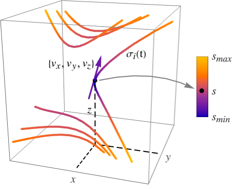
- ListStreamPlot3Dは,3Dストリームプロットあるいは流線プロットとして知られている.流線は,線の他に管(ストリームチューブ)やリボン(ストリームリボン)として表示することもできる.
- ListStreamPlot3Dは,
 および
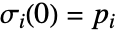 で定義された流線
 をプロットする.ただし,
 はベクトルデータの補間関数で,
 は初期流点である.流線
 は点
 を通る曲線で,その接線は各点におけるベクトル場
 に対応する.
- 流線は,デフォルトで,ベクトル場
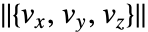 の強度
 に従って彩色され,矢印は
 が大きくなる方向を向く.
- ベクトル場
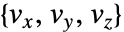 は
 で値 varr〚i,j,k〛を持つ.
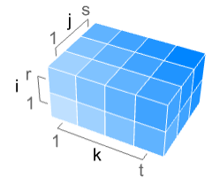
- varr は立体内のベクトルを表す.デフォルトで,点{k,j,i}はベクトル varr〚i,j,k〛を持つと解釈される.ただし,次元{r,s,t,3}の任意の配列について 1≤i≤r,1≤j≤s,1≤k≤t である.
- ListStreamPlot3Dは,デフォルトで,プロット全体を均一な密度にするために十分な流線を表示する.背景のスカラー場は表示しない.
- ListStreamPlot3Dには,Graphics3Dと同じオプションに以下の追加・変更を加えたものが使える. [全オプションのリスト]
-
BoxRatios {1,1,1} 高さと幅の割合 Method Automatic プロットに使用するメソッド PerformanceGoal $PerformanceGoal 最適化しようとするパフォーマンスの局面 PlotLegends None 含める凡例 PlotRange {Full,Full,Full} 含める x, y, z の値の範囲 PlotRangePadding Automatic 値の範囲をどの程度充填するか PlotTheme $PlotTheme プロットの全体的なテーマ RegionBoundaryStyle Automatic プロット領域の境界のスタイル RegionFunction True& 含める領域を決定する ScalingFunctions None 個々の座標のスケール方法 StreamColorFunction Automatic 流線の彩色方法 StreamColorFunctionScaling True StreamColorFunctionの引数をスケールするかどうか StreamMarkers Automatic 流れに使用する形状 StreamPoints Automatic 流線の数または配置 StreamScale None 流線のサイズのスケール方法 StreamStyle Automatic 流線の描画方法 - RegionFunctionおよびColorFunctionの中の関数に渡される引数は x,y,z,vx,vy,vz,Norm[{vx,vy,vz}]である.
- 次は,StreamMarkersの可能な設定である.
-

"Arrow" 2Dの鏃を持つ線 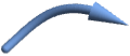
"Arrow3D" 3Dの鏃を持つ管 
"Line" 線 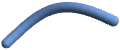
"Tube" 管 
"Ribbon" 平らなリボン 
"ArrowRibbon" 組込みの鏃を持つリボン - StreamScaleAutomaticで「矢印」流線マーカーを使うと,流線の方向が分かりやすくなるように,流線が線分に分割される.
- 次は,StreamScaleの可能な設定である.
-
Automatic 流線の線分を自動的に決める Full 流線全体を分割せずに使う Tiny,Small,Medium,Large 線分の長さを指定する名前付きの設定 {len,npts,ratio} 流線の線分に明示的な指定を使う - 流線線分の長さ len は以下のいずれの形でもよい.
-
Automatic 長さを自動的に決定する None 流線を一まとまりで表示する Tiny,Small,Medium,Large 名前付きの線分長を使う s グラフィックスサイズとの割合の長さ s - 各線分を描画するための点の数 npts は,Automaticまたは特定の点の数でよい.
- 縦横比 ratio は流線線分と相対的な流線の横断面の幅を指定する.
- 次は,ScalingFunctionsの可能な設定である.
-
{sx,sy,sz} x,y,z の各軸をスケールする - 次は,よく使われる組込みのスケーリング関数 s である.
-
"Log" 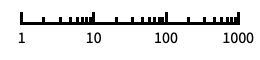
自動目盛ラベル付きの対数スケール "Log10" 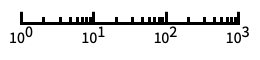
10のベキ乗に目盛が付いた,10を底とする対数スケール "SignedLog" 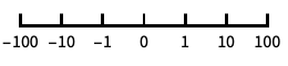
0と負の数を含む対数に似たスケール "Reverse" 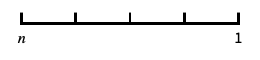
座標の向きを逆にする "Infinite" 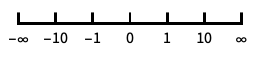
無限スケール
全オプションのリスト
例題
すべて開く すべて閉じる例 (4)
指定されたベクトル集合から補間されたベクトル場をプロットする:
ListStreamPlot3D[Table[{z, -x, y}, {x, -1, 1, .1}, {y, -1, 1, .1}, {z, -1, 1, .1}]]ListStreamPlot3D[Table[{x + y, y - z, x}, {x, -1, 1, .1}, {y, -1, 1, .1}, {z, -1, 1, .1}], PlotLegends -> Automatic]ListStreamPlot3D[Table[{x, y + z, z}, {x, -1, 1, .1}, {y, -1, 1, .1}, {z, -1, 1, .1}], StreamMarkers -> "Tube"]ListStreamPlot3D[Table[{x, y, 1 + 2y}, {x, -1, 1, .1}, {y, -1, 1, .1}, {z, -1, 1, .1}], DataRange -> {{-1, 1}, {-1, 1}, {-1, 1}}]スコープ (12)
サンプリング (3)
ListStreamPlot3D[Table[{2 , -Sin[π x], -x}, {x, -1, 1, 0.1}, {y, -1, 1, 0.1}, {z, -1, 1, 0.1}], StreamPoints -> Coarse]ListStreamPlot3D[Table[{2 , -Sin[π x], -x}, {x, -1, 1, 0.1}, {y, -1, 1, 0.1}, {z, -1, 1, 0.1}], StreamPoints -> RandomReal[{1, 20}, {30, 3}]]ListStreamPlot3D[Table[{2 , -Sin[π x], -x}, {x, -1, 1, 0.1}, {y, -1, 1, 0.1}, {z, -1, 1, 0.1}], RegionFunction -> Function[{x, y, z}, y ≥ x]]プレゼンテーション (9)
ListStreamPlot3D[Table[{x, y, 1 + 2y}, {x, -1, 1, 0.1}, {y, -1, 1, 0.1}, {z, -1, 1, 0.1}]]ListStreamPlot3D[Table[{x, y, 1 + 2y}, {x, -1, 1, 0.1}, {y, -1, 1, 0.1}, {z, -1, 1, 0.1}], StreamMarkers -> "Tube"]ListStreamPlot3D[Table[{x, y, 1 + 2y}, {x, -1, 1, 0.1}, {y, -1, 1, 0.1}, {z, -1, 1, 0.1}], StreamMarkers -> "Ribbon"]流線マーカーの「矢印」バージョンを使って流線に沿った流れの方向を示す:
ListStreamPlot3D[Table[{x, y, 1 + 2y}, {x, -1, 1, 0.1}, {y, -1, 1, 0.1}, {z, -1, 1, 0.1}], StreamMarkers -> "Arrow"]ListStreamPlot3D[Table[{x, y, 1 + 2y}, {x, -1, 1, 0.1}, {y, -1, 1, 0.1}, {z, -1, 1, 0.1}], StreamMarkers -> "Arrow3D"]リボンは,流線の頭を先細りにし,尾を切り欠くことによって矢印に変えられる:
ListStreamPlot3D[Table[{x, y, 1 + 2y}, {x, -1, 1, 0.1}, {y, -1, 1, 0.1}, {z, -1, 1, 0.1}], StreamMarkers -> "ArrowRibbon"]ListStreamPlot3D[Table[{x, y, 1 + 2y}, {x, -1, 1, 0.1}, {y, -1, 1, 0.1}, {z, -1, 1, 0.1}], StreamColorFunction -> None, StreamStyle -> RGBColor[0.09, 0.76, 0.65], StreamMarkers -> "Tube"]ListStreamPlot3D[Table[{x, y, 1 + 2y}, {x, -1, 1, 0.1}, {y, -1, 1, 0.1}, {z, -1, 1, 0.1}], StreamColorFunction -> "Rainbow"]ListStreamPlot3D[Table[{x, y, 1 + 2y}, {x, -1, 1, 0.1}, {y, -1, 1, 0.1}, {z, -1, 1, 0.1}], PlotLegends -> Automatic]StreamScaleを使って流線をより短い複数の線分に分割する:
ListStreamPlot3D[Table[{x, y, 1 + 2y}, {x, -1, 1, 0.1}, {y, -1, 1, 0.1}, {z, -1, 1, 0.1}], StreamScale -> 0.1]ListStreamPlot3D[Table[{x, y, 1 + 2y}, {x, -1, 1, 0.1}, {y, -1, 1, 0.1}, {z, -1, 1, 0.1}], StreamScale -> 0.2]ListStreamPlot3D[Table[{x, y, 1 + 2y}, {x, -1, 1, 0.1}, {y, -1, 1, 0.1}, {z, -1, 1, 0.1}], StreamMarkers -> "Arrow", StreamScale -> {Full, 20, 0.2}]ListStreamPlot3D[Table[{x, y, 1 + 2y}, {x, -1, 1, 0.1}, {y, -1, 1, 0.1}, {z, -1, 1, 0.1}], PlotTheme -> "Marketing"]ListStreamPlot3D[Table[{x, y, 1 + 2y}, {x, -1, 1, 0.1}, {y, -1, 1, 0.1}, {z, -1, 1, 0.1}], ScalingFunctions -> {None, None, "Log"}]オプション (75)
Axes (3)
デフォルトで,Axesが描かれる:
ListStreamPlot3D[Table[{x, 2y, 3z}, {x, -2, 2, 0.1}, {y, -1, 1, 0.1}, {z, -1, 1, 0.1}]]ListStreamPlot3D[Table[{x, 2y, 3z}, {x, -2, 2, 0.1}, {y, -1, 1, 0.1}, {z, -1, 1, 0.1}], Axes -> False]{ListStreamPlot3D[Table[{x, 2y, 3z}, {x, -2, 2, 0.1}, {y, -1, 1, 0.1}, {z, -1, 1, 0.1}], Axes -> {True, False, False}], ListStreamPlot3D[Table[{x, 2y, 3z}, {x, -2, 2, 0.1}, {y, -1, 1, 0.1}, {z, -1, 1, 0.1}], Axes -> {False, True, False}], ListStreamPlot3D[Table[{x, 2y, 3z}, {x, -2, 2, 0.1}, {y, -1, 1, 0.1}, {z, -1, 1, 0.1}], Axes -> {False, False, True}]}AxesLabel (4)
ListStreamPlot3D[Table[{x, 2y, 3z}, {x, -2, 2, 0.1}, {y, -1, 1, 0.1}, {z, -1, 1, 0.1}]]
ListStreamPlot3D[Table[{x, 2y, 3z}, {x, -2, 2, 0.1}, {y, -1, 1, 0.1}, {z, -1, 1, 0.1}], AxesLabel -> z]ListStreamPlot3D[Table[{x, 2y, 3z}, {x, -2, 2, 0.1}, {y, -1, 1, 0.1}, {z, -1, 1, 0.1}], AxesLabel -> {x, y, z}]ListStreamPlot3D[QuantityArray[Table[{x, 2y, 3z}, {x, -2, 2, 0.1}, {y, -1, 1, 0.1}, {z, -1, 1, 0.1}], "Meters"], AxesLabel -> Automatic]AxesOrigin (2)
AxesStyle (4)
ListStreamPlot3D[Table[{x, 2y, 3z}, {x, -2, 2, 0.1}, {y, -1, 1, 0.1}, {z, -1, 1, 0.1}], AxesStyle -> StandardRed]ListStreamPlot3D[Table[{x, 2y, 3z}, {x, -2, 2, 0.1}, {y, -1, 1, 0.1}, {z, -1, 1, 0.1}], AxesStyle -> {{Thick, StandardBrown}, {Thick, StandardBlue}, {Thick, StandardGreen}}]ListStreamPlot3D[Table[{x, 2y, 3z}, {x, -2, 2, 0.1}, {y, -1, 1, 0.1}, {z, -1, 1, 0.1}], AxesStyle -> StandardGreen, TicksStyle -> StandardGray]ListStreamPlot3D[Table[{x, 2y, 3z}, {x, -2, 2, 0.1}, {y, -1, 1, 0.1}, {z, -1, 1, 0.1}], AxesStyle -> StandardGreen, LabelStyle -> StandardGray]BoxRatios (2)
DataRange (2)
デフォルトで,データ範囲はデータ配列の指標範囲であるとみなされる:
ListStreamPlot3D[Table[{x - y, y - z, z - x}, {x, -2, 2, 0.1}, {y, -1, 1, 0.1}, {z, -1, 1, 0.1}]]ListStreamPlot3D[Table[{x - y, y - z, z - x}, {x, -2, 2, 0.1}, {y, -1, 1, 0.1}, {z, -1, 1, 0.1}], DataRange -> {{-2, 2}, {-1, 1}, {-1, 1}}]ImageSize (7)
Tiny,Small,Medium,Largeのような名前付きのサイズを使う:
{ListStreamPlot3D[Table[{x, 2y, 3z}, {x, -2, 2, 0.1}, {y, -1, 1, 0.1}, {z, -1, 1, 0.1}], ImageSize -> Tiny], ListStreamPlot3D[Table[{x, 2y, 3z}, {x, -2, 2, 0.1}, {y, -1, 1, 0.1}, {z, -1, 1, 0.1}], ImageSize -> Small]}{ListStreamPlot3D[Table[{x, 2y, 3z}, {x, -2, 2, 0.1}, {y, -1, 1, 0.1}, {z, -1, 1, 0.1}], ImageSize -> 150], ListStreamPlot3D[Table[{x, 2y, 3z}, {x, -2, 2, 0.1}, {y, -1, 1, 0.1}, {z, -1, 1, 0.1}], AspectRatio -> 1.5, ImageSize -> 150]}{ListStreamPlot3D[Table[{x, 2y, 3z}, {x, -2, 2, 0.1}, {y, -1, 1, 0.1}, {z, -1, 1, 0.1}], ImageSize -> {Automatic, 150}], ListStreamPlot3D[Table[{x, 2y, 3z}, {x, -2, 2, 0.1}, {y, -1, 1, 0.1}, {z, -1, 1, 0.1}], AspectRatio -> 2, ImageSize -> {Automatic, 150}]}{ListStreamPlot3D[Table[{x, 2y, 3z}, {x, -2, 2, 0.1}, {y, -1, 1, 0.1}, {z, -1, 1, 0.1}], ImageSize -> UpTo[200]], ListStreamPlot3D[Table[{x, 2y, 3z}, {x, -2, 2, 0.1}, {y, -1, 1, 0.1}, {z, -1, 1, 0.1}], AspectRatio -> 2, ImageSize -> UpTo[200]]}グラフィックスの幅と高さを指定して,必要な場合はスペースで充填する:
ListStreamPlot3D[Table[{x, 2y, 3z}, {x, -2, 2, 0.1}, {y, -1, 1, 0.1}, {z, -1, 1, 0.1}], ImageSize -> {200, 300}, Background -> StandardBlue]AspectRatioFullと設定すると,使用可能なスペースが塗り潰される:
ListStreamPlot3D[Table[{x, 2y, 3z}, {x, -2, 2, 0.1}, {y, -1, 1, 0.1}, {z, -1, 1, 0.1}], AspectRatio -> Full, ImageSize -> {200, 300}, Background -> StandardBlue]{ListStreamPlot3D[Table[{x, 2y, 3z}, {x, -2, 2, 0.1}, {y, -1, 1, 0.1}, {z, -1, 1, 0.1}], ImageSize -> {UpTo[150], UpTo[100]}], ListStreamPlot3D[Table[{x, 2y, 3z}, {x, -2, 2, 0.1}, {y, -1, 1, 0.1}, {z, -1, 1, 0.1}], AspectRatio -> 2, ImageSize -> {UpTo[150], UpTo[100]}]}ImageSizeFullを使ってオブジェクト内の使用可能なスペースを塗り潰す:
Framed[Pane[ListStreamPlot3D[Table[{x, 2y, 3z}, {x, -2, 2, 0.1}, {y, -1, 1, 0.1}, {z, -1, 1, 0.1}], ImageSize -> Full, Background -> StandardBlue], {200, 100}]]Framed[Pane[ListStreamPlot3D[Table[{x, 2y, 3z}, {x, -2, 2, 0.1}, {y, -1, 1, 0.1}, {z, -1, 1, 0.1}], AspectRatio -> Full, ImageSize -> {Scaled[0.5], Scaled[0.5]}, Background -> StandardBlue], {200, 200}]]PlotLegends (3)
ListStreamPlot3D[Table[{1 - x, y - x, z - y}, {x, -1, 1, 0.1}, {y, -1, 1, 0.1}, {z, -1, 1, 0.1}]]ListStreamPlot3D[Table[{1 - x, y - x, z - y}, {x, -1, 1, 0.1}, {y, -1, 1, 0.1}, {z, -1, 1, 0.1}], PlotLegends -> Automatic]ListStreamPlot3D[Table[{1 - x, y - x, z - y}, {x, -1, 1, 0.1}, {y, -1, 1, 0.1}, {z, -1, 1, 0.1}], PlotLegends -> Placed[Automatic, Left]]PlotTheme (1)
RegionBoundaryStyle (4)
RegionFunctionで定義された範囲を表示する:
ListStreamPlot3D[Table[{1, -z, y}, {x, -2, 2, 0.5}, {y, -2, 2, 0.5}, {z, -2, 2, 0.5}], RegionFunction -> Function[{x, y, z, vx, vy, vz, n}, n < 2]]Noneを使って境界を表示しないようにする:
ListStreamPlot3D[Table[{1, -z, y}, {x, -2, 2, 0.5}, {y, -2, 2, 0.5}, {z, -2, 2, 0.5}], RegionFunction -> Function[{x, y, z, vx, vy, vz, n}, n < 2], RegionBoundaryStyle -> None]ListStreamPlot3D[Table[{1, -z, y}, {x, -2, 2, 0.5}, {y, -2, 2, 0.5}, {z, -2, 2, 0.5}], RegionFunction -> Function[{x, y, z, vx, vy, vz, n}, n < 2], RegionBoundaryStyle -> Yellow]ListStreamPlot3D[Table[{1, -z, y}, {x, -2, 2, 0.5}, {y, -2, 2, 0.5}, {z, -2, 2, 0.5}]]RegionFunction (4)
ListStreamPlot3D[Table[{y, -x, 3}, {x, -5, 5}, {y, -5, 5}, {z, -5, 5}], RegionFunction -> Function[{x, y, z, vx, vy, vz, n}, vx vy ≥ 0]]場の大きさが与えられた閾値を超えるところにのみ流れをプロットする:
ListStreamPlot3D[Table[{y, -x, 3}, {x, -5, 5}, {y, -5, 5}, {z, -5, 5}], RegionFunction -> Function[{x, y, z, vx, vy, vz, n}, n ≥ 5]]ListStreamPlot3D[Table[{y, -x, 3}, {x, -5, 5}, {y, -5, 5}, {z, -5, 5}], RegionFunction -> Function[{x, y, z, vx, vy, vz, n}, 3n ≥ x + y]]RegionBoundaryStyleNoneを使って境界を表示しないようにする:
ListStreamPlot3D[Table[{y, -x, 3}, {x, -5, 5}, {y, -5, 5}, {z, -5, 5}], RegionFunction -> Function[{x, y, z, vx, vy, vz, n}, n ≥ 5], RegionBoundaryStyle -> None]ScalingFunctions (3)
ListStreamPlot3D[Table[{x, y, 1 + 2y}, {x, -1, 1, 0.1}, {y, -1, 1, 0.1}, {z, -1, 1, 0.1}]]ListStreamPlot3D[Table[{x, y, 1 + 2y}, {x, -1, 1, 0.1}, {y, -1, 1, 0.1}, {z, -1, 1, 0.1}], ScalingFunctions -> {None, None, "Log"}]ListStreamPlot3D[Table[{x, y, 1 + 2y}, {x, -1, 1, 0.1}, {y, -1, 1, 0.1}, {z, -1, 1, 0.1}], ScalingFunctions -> {None, None, "Reverse"}]StreamColorFunction (4)
ListStreamPlot3D[Table[{3x, 2y, z}, {x, -1, 1, 0.1}, {y, -1, 1, 0.1}, {z, -1, 1, 0.1}], StreamColorFunction -> Hue]ColorDataからの任意の名前付き色勾配を使う:
ListStreamPlot3D[Table[{3x, 2y, z}, {x, -1, 1, 0.1}, {y, -1, 1, 0.1}, {z, -1, 1, 0.1}], StreamColorFunction -> "Rainbow"]ListStreamPlot3D[Table[{3x, 2y, z}, {x, -1, 1, 0.1}, {y, -1, 1, 0.1}, {z, -1, 1, 0.1}], StreamColorFunction -> Function[{x, y, z, vx, vy, vz, n}, Hue[x]]]StreamColorFunctionScalingFalseを使ってスケールされていない値を得る:
ListStreamPlot3D[Table[{3x, 2y, z}, {x, -1, 1, 0.1}, {y, -1, 1, 0.1}, {z, -1, 1, 0.1}], StreamColorFunction -> "Rainbow", StreamColorFunctionScaling -> False]StreamColorFunctionScaling (2)
ListStreamPlot3D[Table[{y, -x, E^z}, {x, -1, 1, 0.1}, {y, -1, 1, 0.1}, {z, -1, 1, 0.1}], StreamColorFunction -> "Pastel", PlotLegends -> Automatic]StreamColorFunctionScalingFalseを使ってスケールされていない値を得る:
ListStreamPlot3D[Table[{y, -x, E^z}, {x, -1, 1, 0.1}, {y, -1, 1, 0.1}, {z, -1, 1, 0.1}], StreamColorFunction -> "Pastel", PlotLegends -> Automatic, StreamColorFunctionScaling -> False]StreamMarkers (5)
ListStreamPlot3D[Table[{E^x, E^y, -3}, {x, -1, 1, 0.1}, {y, -1, 1, 0.1}, {z, -1, 1, 0.1}]]ListStreamPlot3D[Table[{E^x, E^y, -3}, {x, -1, 1, 0.1}, {y, -1, 1, 0.1}, {z, -1, 1, 0.1}], StreamMarkers -> "Tube"]ListStreamPlot3D[Table[{E^x, E^y, -3}, {x, -1, 1, 0.1}, {y, -1, 1, 0.1}, {z, -1, 1, 0.1}], StreamMarkers -> "Ribbon"]"Arrow"流れマーカーは,流線を自動的により短い線分に分割する:
ListStreamPlot3D[Table[{E^x, E^y, -3}, {x, -1, 1, 0.1}, {y, -1, 1, 0.1}, {z, -1, 1, 0.1}], StreamMarkers -> "Arrow"]ListStreamPlot3D[Table[{E^x, E^y, -3}, {x, -1, 1, 0.1}, {y, -1, 1, 0.1}, {z, -1, 1, 0.1}], StreamMarkers -> "Arrow3D"]ListStreamPlot3D[Table[{E^x, E^y, -3}, {x, -1, 1, 0.1}, {y, -1, 1, 0.1}, {z, -1, 1, 0.1}], StreamMarkers -> "ArrowRibbon"]ListStreamPlot3D[Table[{E^x, E^y, -3}, {x, -1, 1, 0.1}, {y, -1, 1, 0.1}, {z, -1, 1, 0.1}], StreamMarkers -> "Arrow3D", StreamScale -> Full]ListStreamPlot3D[Table[{E^x, E^y, -3}, {x, -1, 1, 0.1}, {y, -1, 1, 0.1}, {z, -1, 1, 0.1}], StreamMarkers -> "Ribbon", StreamScale -> 0.1]StreamPoints (4)
ListStreamPlot3D[Table[{1, -E^-y, E^z}, {x, -2, 2, 0.1}, {y, -2, 2, 0.1}, {z, -2, 2, 0.1}]]ListStreamPlot3D[Table[{1, -E^-y, E^z}, {x, -2, 2, 0.1}, {y, -2, 2, 0.1}, {z, -2, 2, 0.1}], StreamPoints -> 40]ListStreamPlot3D[Table[{1, -E^-y, E^z}, {x, -2, 2, 0.1}, {y, -2, 2, 0.1}, {z, -2, 2, 0.1}], StreamPoints -> RandomReal[{1, 40}, {20, 3}]]ListStreamPlot3D[Table[{1, -E^-y, E^z}, {x, -2, 2, 0.1}, {y, -2, 2, 0.1}, {z, -2, 2, 0.1}], StreamPoints -> Coarse]ListStreamPlot3D[Table[{1, -E^-y, E^z}, {x, -2, 2, 0.1}, {y, -2, 2, 0.1}, {z, -2, 2, 0.1}], StreamPoints -> Fine]StreamScale (9)
分割されたマーカーにはデフォルトの長さ,点の数,縦横比がある:
ListStreamPlot3D[Table[{y^2, -x^2, 2 - z}, {x, -1, 1, 0.1}, {y, -1, 1, 0.1}, {z, -1, 1, 0.1}], StreamMarkers -> "Arrow"]ListStreamPlot3D[Table[{y^2, -x^2, 2 - z}, {x, -1, 1, 0.1}, {y, -1, 1, 0.1}, {z, -1, 1, 0.1}], StreamMarkers -> "Arrow", StreamScale -> 0.2]ListStreamPlot3D[Table[{y^2, -x^2, 2 - z}, {x, -1, 1, 0.1}, {y, -1, 1, 0.1}, {z, -1, 1, 0.1}], StreamMarkers -> "Arrow", StreamScale -> {0.2, 2}]ListStreamPlot3D[Table[{y^2, -x^2, 2 - z}, {x, -1, 1, 0.1}, {y, -1, 1, 0.1}, {z, -1, 1, 0.1}], StreamMarkers -> "Arrow", StreamScale -> {0.2, 2, 0.2}]ListStreamPlot3D[Table[{y^2, -x^2, 2 - z}, {x, -1, 1, 0.1}, {y, -1, 1, 0.1}, {z, -1, 1, 0.1}], StreamMarkers -> "Arrow", StreamScale -> Full]ListStreamPlot3D[Table[{y^2, -x^2, 2 - z}, {x, -1, 1, 0.1}, {y, -1, 1, 0.1}, {z, -1, 1, 0.1}], StreamMarkers -> "Ribbon", StreamScale -> 0.2]ListStreamPlot3D[Table[{y^2, -x^2, 2 - z}, {x, -1, 1, 0.1}, {y, -1, 1, 0.1}, {z, -1, 1, 0.1}], StreamMarkers -> "ArrowRibbon", StreamScale -> {Automatic, Automatic, 0.05}]ListStreamPlot3D[Table[{y^2, -x^2, 2 - z}, {x, -1, 1, 0.1}, {y, -1, 1, 0.1}, {z, -1, 1, 0.1}], StreamMarkers -> "Ribbon", StreamScale -> {Automatic, Automatic, 0.05}]ListStreamPlot3D[Table[{y^2, -x^2, 2 - z}, {x, -1, 1, 0.1}, {y, -1, 1, 0.1}, {z, -1, 1, 0.1}], StreamMarkers -> "Tube", StreamScale -> {Automatic, Automatic, 0.05}]ListStreamPlot3D[Table[{y^2, -x^2, 2 - z}, {x, -1, 1, 0.1}, {y, -1, 1, 0.1}, {z, -1, 1, 0.1}], StreamMarkers -> "Arrow", StreamScale -> {Automatic, Automatic, 0.2}]ListStreamPlot3D[Table[{y^2, -x^2, 2 - z}, {x, -1, 1, 0.1}, {y, -1, 1, 0.1}, {z, -1, 1, 0.1}], StreamMarkers -> "Arrow", StreamScale -> {0.5, 3}]StreamStyle (3)
ListStreamPlot3D[Table[{-y^2, x^2, 0.5}, {x, -1, 1, 0.1}, {y, -1, 1, 0.1}, {z, -1, 1, 0.1}], StreamStyle -> Thickness[0.02]]StreamColorFunctionはStreamStyleより優先順位が高い:
ListStreamPlot3D[Table[{-y^2, x^2, 0.5}, {x, -1, 1, 0.1}, {y, -1, 1, 0.1}, {z, -1, 1, 0.1}], StreamStyle -> Directive[Red, Dashing[{0.1, 0.02}]]]StreamColorFunctionNoneを使ってStreamStyleで流線の色を指定する:
ListStreamPlot3D[Table[{-y^2, x^2, 0.5}, {x, -1, 1, 0.1}, {y, -1, 1, 0.1}, {z, -1, 1, 0.1}], StreamStyle -> Directive[StandardRed, Dashing[{0.1, 0.02}]], StreamColorFunction -> None]Ticks (6)
ListStreamPlot3D[Table[{x + y, y - z, x}, {z, -2, 2, 0.1}, {y, -2, 2, 0.1}, {x, -2, 2, 0.1}]]ListStreamPlot3D[Table[{x + y, y - z, x}, {z, -2, 2, 0.1}, {y, -2, 2, 0.1}, {x, -2, 2, 0.1}], Ticks -> None]ListStreamPlot3D[Table[{x + y, y - z, x}, {z, -2, 2, 0.1}, {y, -2, 2, 0.1}, {x, -2, 2, 0.1}], Ticks -> {{5, 15, 25}, {5, 15, 25}, {5, 15, 25}}]ListStreamPlot3D[Table[{x + y, y - z, x}, {z, -2, 2, 0.1}, {y, -2, 2, 0.1}, {x, -2, 2, 0.1}], Ticks -> {{{5, a}, {15, b}, {25, c}}, {{5, a}, {15, b}, {25, c}}, {{5, a}, {15, b}, {25, c}}}]ListStreamPlot3D[Table[{x + y, y - z, x}, {z, -2, 2, 0.1}, {y, -2, 2, 0.1}, {x, -2, 2, 0.1}], Ticks -> {{{5, a, .1}, {15, b, .1}, {25, c, .1}}, {{5, a, .05}, {15, b, .05}, {25, c, .05}}, {{5, a, .15}, {15, b, .15}, {25, c, .15}}}]ListStreamPlot3D[Table[{x + y, y - z, x}, {z, -2, 2, 0.1}, {y, -2, 2, 0.1}, {x, -2, 2, 0.1}], Ticks -> {{{5, a, .1, Directive[Red]}, {15, b, .1, Directive[Red, Thick]}, {25, c, .1, Directive[Red, Dashed, Thick]}}, {{5, a, .1, Directive[Blue]}, {15, b, .1, Directive[Blue, Thick]}, {25, c, .1, Directive[Blue, Dashed, Thick]}}, {{5, a, .1, Directive[Darker@Green]}, {15, b, .1, Directive[Darker@Green, Thick]}, {25, c, .1, Directive[Darker@Green, Dashed, Thick]}}}]TicksStyle (3)
デフォルトで,目盛と目盛ラベルには軸と同じスタイルが使われる:
ListStreamPlot3D[Table[{x + y, y - z, x}, {z, -2, 2, 0.1}, {y, -2, 2, 0.1}, {x, -2, 2, 0.1}], AxesStyle -> Directive[Thick, StandardRed]]ListStreamPlot3D[Table[{x + y, y - z, x}, {z, -2, 2, 0.1}, {y, -2, 2, 0.1}, {x, -2, 2, 0.1}], TicksStyle -> Directive[Bold, StandardRed]]ListStreamPlot3D[Table[{x + y, y - z, x}, {z, -2, 2, 0.1}, {y, -2, 2, 0.1}, {x, -2, 2, 0.1}], TicksStyle -> {Directive[StandardGray, Bold], Directive[Bold, StandardRed], Directive[Bold, StandardBlue]}]アプリケーション (2)
等しい一定の電荷密度と反対の符号を持つ有限長の2本の細いワイヤーの影響下にある点のサンプリングで電場を数値的に計算する:
data = Quiet@Table[If[Abs[x] == 1 && z == 0 && -2 ≤ y ≤ 2, {0, 0, 0}, NIntegrate[({x + 1, y - Y, z}/Norm[{x + 1, y - Y, z}]^3) - ({x - 1, y - Y, z}/Norm[{x - 1, y - Y, z}]^3), {Y, -2, 2}]], {x, -5, 5}, {y, -5, 5}, {z, -5, 5}];正の電荷(黒)と負の電荷(赤)のワイヤーと一緒に電場を可視化する:
Show[ListStreamPlot3D[data, StreamMarkers -> "Arrow", DataRange -> {{-5, 5}, {-5, 5}, {-5, 5}}, StreamColorFunction -> None, StreamStyle -> StandardBlue], Graphics3D[{Thickness[0.01], Line[{{-1, -2, 0}, {-1, 2, 0}}], StandardRed, Line[{{1, -2, 0}, {1, 2, 0}}]}]]単位立方体内の時間依存の熱流を可視化する.単位立方体の温度が  のときの定常状態熱方程式
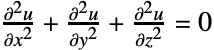 について考える.ただし,以下に示すように,
 面で
 ,
 ,
 ,
 ,
 の各面は断熱,
 面の半径0.3の円板を中心とする内部は
 .円板の外は
 とする:
cube = [image];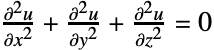
n = 20; (* number of steps *)
Δ = (1.0/n + 1); (* step size *)
vars = Flatten[Table[u[i, j, k], {i, 1, n}, {j, 0, n + 1}, {k, 0, n + 1}]];
eqns = Flatten[Table[
	u[i + 1, j, k] - 2u[i, j, k] + u[i - 1, j, k] + (* x direction *)
	u[i, j + 1, k] - 2u[i, j, k] + u[i, j - 1, k] + (* y direction *)
	u[i, j, k + 1] - 2u[i, j, k] + u[i, j, k - 1](* z direction *)
	 == 0, {i, 1, n}, {j, 0, n + 1}, {k, 0, n + 1}]];


u[0, _, _] := 1.0;
u[n + 1, j_, k_] := If[(j Δ - 0.5)^2 + (k Δ - 0.5)^2 ≤ 0.3^2, 2, 0];
u[i_, -1, k_] := u[i, 1, k];(* y=0 *)
u[i_, n + 2, k_] := u[i, n, k]; (* y=1 *)
u[i_, j_, -1] := u[i, j, 1]; (* z=0 *)
u[i_, j_, n + 2] := u[i, j, n];(* z=1 *)sol = Solve[eqns, vars][[1]];
temperatures = Table[u[i, j, k], {k, 0, n + 1}, {j, 0, n + 1}, {i, 0, n + 1}] /. sol;heatflux = Table[-{(u[i + 1, j, k] - u[i - 1, j, k]/2Δ), (u[i, j + 1, k] - u[i, j - 1, k]/2Δ), (u[i, j, k + 1] - u[i, j, k - 1]/2Δ)} /. sol, {i, 1, n}, {j, 1, n}, {k, 1, n}];
sp1 = Flatten[Table[{0, y, z}, {y, 0.1, 0.9, 0.2}, {z, 0.1, 0.9, 0.2}], 1];
sp2 = Flatten[Table[{1, 0.5 + r Cos[t], 0.5 + r Sin[t]}, {r, 0, 0.2, 0.1}, {t, 0, 2π - (π/5), (π/5)}], 1];熱流を可視化する.境界温度は凡例で指定されており,立方体の空白の面は断熱されている:
Show[ListStreamPlot3D[heatflux, DataRange -> {{0, 1}, {0, 1}, {0, 1}}, StreamPoints -> Join[sp1, sp2], StreamMarkers -> "Arrow3D", StreamScale -> Full, StreamColorFunction -> None, StreamStyle -> RGBColor[0.8675693999999999, 0.4915453999999999, 0.21120899999999998]], cube, Lighting -> "Neutral"]特性と関係 (10)
StreamPlot3DとVectorPlot3Dを使って関数を可視化する:
{StreamPlot3D[{z, -x, y}, {x, -3, 3}, {y, -3, 3}, {z, -3, 3}], VectorPlot3D[{z, -x, y}, {x, -3, 3}, {y, -3, 3}, {z, -3, 3}]}StreamPlotおよびVectorPlotを使って関数を2Dで可視化する:
{StreamPlot[{y - x, y}, {x, -3, 3}, {y, -3, 3}], VectorPlot[{y - x, y}, {x, -3, 3}, {y, -3, 3}]}ListSliceVectorPlot3Dで曲面に沿ってベクトルをプロットする:
data = Table[{-1 - x ^ 2 + y, 1 + x - y ^ 2, z}, {x, -3, 3}, {y, -3, 3}, {z, -3, 3}];ListSliceVectorPlot3D[data]ListVectorPlot3Dを使って3Dの場を離散ベクトルとしてプロットする:
data = Table[{-1 - x ^ 2 + y, 1 + x - y ^ 2, z}, {x, -3, 3}, {y, -3, 3}, {z, -3, 3}];ListVectorPlot3D[data]2DベクトルのプロットにListVectorPlotに使う:
data = Table[{-1 - x ^ 2 + y, 1 + x - y ^ 2}, {x, -3, 3}, {y, -3, 3}];ListVectorPlot[data]ListStreamPlotを使ってベクトルではなく流線をプロットする:
data = Table[{-1 - x ^ 2 + y, 1 + x - y ^ 2}, {x, -3, 3}, {y, -3, 3}];ListStreamPlot[data]ListVectorDensityPlotまたはListStreamDensityPlotを使ってスカラー場の密度プロットを加える:
data = Table[{{-1 - x ^ 2 + y, 1 + x - y ^ 2}, Abs[x] + Abs[y]}, {x, -3, 3}, {y, -3, 3}];{ListVectorDensityPlot[data], ListStreamDensityPlot[data]}ListVectorDisplacementPlotを使って変位ベクトル場に関連付けられた領域の変形を可視化する:
data2D = Table[{{x, y} = RandomReal[{-1, 1}, {2}], {y, x - x^3}}, {300}];data3D = Table[{{x, y, z} = RandomReal[{0, 1}, {3}], {y, x, -z}}, {300}];ListVectorDisplacementPlot[data2D, Disk[], VectorPoints -> Automatic]ListVectorDisplacementPlot3Dを使って変形を3Dで可視化する:
ListVectorDisplacementPlot3D[data3D, Cuboid[], VectorPoints -> "Boundary"]ListLineIntegralConvolutionPlotを使ってベクトル場の線積分たたみ込みをプロットする:
data = Table[{-1 - x ^ 2 + y, 1 + x - y ^ 2}, {x, -3, 3}, {y, -3, 3}];ListLineIntegralConvolutionPlot[data]GeoVectorPlotを使って地図上にベクトルをプロットする:
GeoVectorPlot[GeoVector[GeoPosition[{{-54.79801473961214, -111.85053058521567},
    {-65.56940402358214, 162.89657500795147}, {-81.67990688759895, -93.36222177594851},
    {7.785750774919734, 95.44840765141487}, {-6.86571958448036, -40.946398330539864},
    { ... 904, "AngularDegrees"]},
   {0.9366099079317551, Quantity[357.70482317743733, "AngularDegrees"]},
   {0.8256817194791912, Quantity[242.07227508889662, "AngularDegrees"]},
{0.2661401145642981, Quantity[152.90003252279325, "AngularDegrees"]}}]]GeoStreamPlotを使ってベクトルの代りに流線をプロットする:
GeoStreamPlot[GeoVector[GeoPosition[{{-54.79801473961214, -111.85053058521567},
    {-65.56940402358214, 162.89657500795147}, {-81.67990688759895, -93.36222177594851},
    {7.785750774919734, 95.44840765141487}, {-6.86571958448036, -40.946398330539864},
    { ... 904, "AngularDegrees"]},
   {0.9366099079317551, Quantity[357.70482317743733, "AngularDegrees"]},
   {0.8256817194791912, Quantity[242.07227508889662, "AngularDegrees"]},
   {0.2661401145642981, Quantity[152.90003252279325, "AngularDegrees"]}}]]
考えられる問題 (2)
管のStreamMarkersはBoxRatiosで変形できる:
data = Table[{2, -10 z - x y, 10 y - x z}, {x, -2π, 2π, π / 5}, {y, -1, 1, 0.1}, {z, -1, 1, 0.1}];ListStreamPlot3D[data, StreamMarkers -> "Tube", DataRange -> {{-2π, 2π}, {-1, 1}, {-1, 1}}]BoxRatiosを注意深く調整して管の変形を防ぐ:
ListStreamPlot3D[data, StreamMarkers -> "Tube", DataRange -> {{-2π, 2π}, {-1, 1}, {-1, 1}}, BoxRatios -> {2π, 1, 1}]"Arrow"と"Arrow3D"の流れマーカーの色は矢印の先頭で決定されるので,長い矢印の場合は色の一貫性がなくなる:
ListStreamPlot3D[Table[{x, y, 1}, {x, -1, 1, 0.1}, {y, -1, 1, 0.1}, {z, -1, 1, 0.1}]]ListStreamPlot3D[Table[{x, y, 1}, {x, -1, 1, 0.1}, {y, -1, 1, 0.1}, {z, -1, 1, 0.1}], StreamMarkers -> "Arrow3D", StreamScale -> Full]テキスト
Wolfram Research (2021), ListStreamPlot3D, Wolfram言語関数, https://reference.wolfram.com/language/ref/ListStreamPlot3D.html (2022年に更新).
CMS
Wolfram Language. 2021. "ListStreamPlot3D." Wolfram Language & System Documentation Center. Wolfram Research. Last Modified 2022. https://reference.wolfram.com/language/ref/ListStreamPlot3D.html.
APA
Wolfram Language. (2021). ListStreamPlot3D. Wolfram Language & System Documentation Center. Retrieved from https://reference.wolfram.com/language/ref/ListStreamPlot3D.html