ArrayPlot[array]
配列の値が正方形の離散的な配列として示されるプロットを生成する.
ArrayPlot
ArrayPlot[array]
配列の値が正方形の離散的な配列として示されるプロットを生成する.
詳細とオプション

- ArrayPlot[array]は,グリッドや表における通常の整列と同じように,デフォルトで array の連続する行をページの下に向かって整列し,連続する列は横方向に整列する. »
- array が0と1を含んでいるとき,1は黒い正方形として,0は白い正方形として表示される.
- ArrayPlotはデフォルトにより,グレースケールで出力を生成する.値ゼロが白になり,正または負の最大値が黒になる. »
- PlotRangeの明示的な設定があると,ArrayPlotはデフォルトで最低値を白く,最大値を黒くする.
- array 中の値は,関連する単位が付いた数量でよい.
- 次の特別入力を使うことができる. »
-
None 背景色 色指示子 指定色 - array が不揃いの場合,短い行は右端を背景色で充填されたものとして扱われる. »
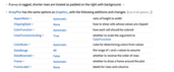
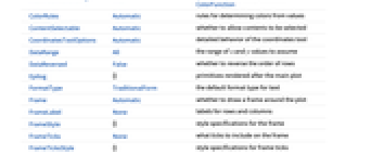
- ArrayPlotはGraphicsと同じオプションに以下の追加・修正を加えたオプションを使うことができる. [全オプションのリスト]
-
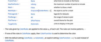
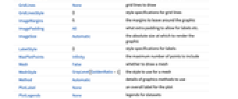
AspectRatio Automatic 縦横比 ClippingStyle None 値が切り取られているセルをどのように表示するか ColorFunction Automatic 各セルをどのように彩色するか ColorFunctionScaling True ColorFunctionの引数をスケールするかどうか ColorRules Automatic 値から色を決定する規則 DataRange All 仮定すべき
と
の値の範囲DataReversed False 行の順序を逆にするかどうか Frame Automatic プロットの周囲に枠を描くかどうか FrameLabel None 行と列のラベル FrameTicks None 枠に入れる目盛 MaxPlotPoints Infinity 含める点の最大数 Mesh False メッシュを描くかどうか MeshStyle GrayLevel[GoldenRatio-1] メッシュに使用するスタイル PlotLegends None データ集合の凡例 PlotRange All プロットする値の範囲 PlotTheme $PlotTheme プロットの全体的なテーマ TargetUnits Automatic プロット中に表示する単位 - ColorRules には,以下の設定を取ることができる.
-
Automatic デフォルトの色を使用する "Colors" 異なる値に対して色を使用する "Monochrome" グレースケールの色を使用する {valcolor,…} color を val のスタイルとして使用する - ColorRulesで与えられる規則は,各セルの値
に適用される.この規則はパターンを含んでいてもよい. » - ColorRulesの規則がどれも適用されなければColorFunctionは色の決定に使われる.
- デフォルト設定のColorRules->Automaticでは,ColorRulesの代りに明示的な設定のColorFunction->f が使われる.
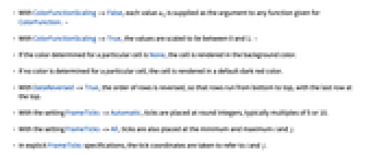
- ColorFunctionScaling->Falseでは,ColorFunctionに与えられた任意の関数に,引数として各値
が渡される. » - ColorFunctionScaling->Trueでは,値は0と1の間に来るようにスケールされる. »
- あるセルに指定された色がNoneの場合,そのセルは背景色で描画される.
- あるセルに色が指定されていない場合,そのセルはデフォルトの暗赤色で描画される.
- DataReversed->Trueの場合,行の順序は逆にされ,最終行が一番上になるように下から上に並べられる.
- FrameTicks->Automaticの設定のとき,目盛は一般に5や10の倍数の整数に四捨五入したところに付けられる.
- FrameTicks->Allの設定のとき,目盛は最小と最大の
と
の位置にも付けれられる. - 明示的なFrameTicks指定では,目盛座標が
と
を参照するものとされる. - DataReversed->Trueの場合,目盛の値は上から下に向けて小さくなっていく.
- PlotRange->amax では,0から amaxまでの間にある
のみが表示される. » - PlotRange->{amin,amax}では,aminから amaxまでの間にある
だけが表示される. - PlotRange->{{imin,imax},{jmin,jmax}}は,指定範囲にある
と
を持った要素のみを表示する.左上の要素は
,
である.デフォルト設定のDataReversed->Falseでは,ページの下に向かうに従って
が増加し,右方向には
が増加する. - PlotRange->{ispec,jspec,aspec}では,指定範囲にある
と
の要素と値だけが表示される. » - ColorFunctionのデフォルト設定のPlotRange->{amin,amax}は,aminから amaxへの値が白から黒へのグレースケールで表示されるように指定する.
- 次は,Meshの可能な設定である.
-
False メッシュラインは描画しない True すべてのセル間にメッシュラインを描画する Automatic もとのセルの周りにだけメッシュラインを描画する "Nonzero" 非零のセルの周りにだけメッシュラインを描画する {mi,mj} i 方向と j 方向にメッシュを指定する - デフォルト設定のFrame->Automaticでは,Mesh->Falseの場合にのみフレームが描かれる.
- 他のグラフィックスと組み合せるために,配列要素
は座標
,
の位置を中心とする単位正方形を覆うと解釈される. - DataRange->{{xmin,xmax},{ymin,ymax}}は,連続するセルの中心を水平方向で xminと xmaxの間に,また垂直方向では yminと ymaxの間に等間隔で置くように指定する.デフォルト設定のDataReversed->Falseでは,
の中心は{xmin,ymax}に置かれる. - デフォルト設定のDataRange->AllでDataReversed->Falseのとき,配列要素
は座標位置
,
を中心とする単位正方形をカバーするものとされる. - ArrayPlotはGraphics[Raster[data],opts]を返す.
- ArrayPlotはSparseArrayオブジェクトと一緒に使うことができる. »
全オプションのリスト
例題
すべて開く すべて閉じる例 (6)
ArrayPlot[{{1, 0, 0, 0.3}, {1, 1, 0, 0.3}, {1, 0, 1, 0.7}}]ArrayPlot[{{1, 0, 0, Pink}, {1, 1, 0, Pink}, {1, 0, 1, Red}}]ArrayPlot[{{1, 0, 0, 0.3}, {1, 1, 0, 0.3}, {1, 0, 1, 0.7}}, ColorRules -> {1 -> Pink, 0 -> Yellow}]ArrayPlot[{{1, 0, 0, 0.3}, {1, 1, 0, 0.3}, {1, 0, 1, 0.7}}, Mesh -> True]ArrayPlot[RandomReal[1, {10, 20}]]ArrayPlot[RandomReal[1, {10, 20}], ColorFunction -> "Rainbow"]スコープ (7)
ArrayPlot[{{-1, 0, 1}, {2, 3, 4}}]ArrayPlot[{{-1, 0, 1}, {2, 3, x}}]ArrayPlot[{{Quantity[0, "Meters"], Quantity[3, "Meters"], Quantity[2, "Meters"], Quantity[9, "Meters"]}, {Quantity[9, "Meters"], Quantity[7, "Meters"], Quantity[3, "Meters"], Quantity[2, "Meters"]}, {Quantity[8, "Meters"], Quantity[8, "Meters"], Quantity[9, "Meters"], Quantity[3, "Meters"]}}]ArrayPlot[RandomChoice[{Red, Green, Blue}, {5, 10}]]ArrayPlot[{{1}, {1, 1}, {1, 0, 1}, {1, 1, 1, 1}}, Background -> Cyan]値がNoneのセルは背景色で描画される:
ArrayPlot[Table[If[x == y, None, 1 / (x - y)], {x, -2, 2}, {y, -2, 2}], Background -> Cyan]ArrayPlot[SparseArray[{{x_, x_} -> 1, ({x_, y_} /; Abs[x - y] < 3) -> .5}, {10, 10}], Mesh -> True]オプション (96)
AspectRatio (2)
Axes (4)
デフォルトで.ArrayPlotは軸の代りに枠を使う:
ArrayPlot[RandomReal[1, {10, 20}]]ArrayPlot[RandomReal[1, {10, 20}], Frame -> False, Axes -> True]AxesOriginを使って軸の交点を指定する:
ArrayPlot[RandomReal[1, {10, 20}], Frame -> False, Axes -> True, AxesOrigin -> {-1, -1}]{ArrayPlot[RandomReal[1, {10, 20}], Frame -> False, Axes -> {True, False}], ArrayPlot[RandomReal[1, {10, 20}], Frame -> False, Axes -> {False, True}]}AxesLabel (3)
ArrayPlot[CellularAutomaton[20, {{1}, 0}, 10], Frame -> False, Axes -> True]ArrayPlot[CellularAutomaton[20, {{1}, 0}, 10], Frame -> False, Axes -> True, AxesLabel -> "Y"]ArrayPlot[CellularAutomaton[20, {{1}, 0}, 10], Frame -> False, Axes -> True, AxesLabel -> {"axis 1", "axes 2"}]AxesOrigin (2)
AxesStyle (4)
ArrayPlot[CellularAutomaton[30, {{1}, 0}, 10], Frame -> False, Axes -> True, AxesStyle -> Red]ArrayPlot[CellularAutomaton[30, {{1}, 0}, 10], Frame -> False, Axes -> True, AxesStyle -> {Directive[Thick, Red], Directive[Thick, Blue]}]ArrayPlot[CellularAutomaton[30, {{1}, 0}, 10], Frame -> False, Axes -> True, AxesStyle -> Red, TicksStyle -> Blue]ArrayPlot[CellularAutomaton[30, {{1}, 0}, 10], Frame -> False, Axes -> True, AxesStyle -> Red, LabelStyle -> Blue]Background (4)
Backgroundは通常辺付近でしか見えない:
ArrayPlot[{{1, 0, 0, 0.3}, {1, 1, 0, 0.3}, {1, 0, 1, 0.7}}, Background -> Blue]明示的な項目がNoneの場合は,背景が「透けて見える」:
ArrayPlot[{{1, 0, 0, None}, {1, 1, 0, None}, {1, None, 1, 0.7}}, Background -> Blue]デフォルトにより,Backgroundはプロット範囲外の値の場合でも背景が透けて見えるようにする:
ArrayPlot[{{1, 0, 0, 0.3}, {1, 1, 0, 0.3}, {1, 0, 1, 0.7}}, Background -> Blue, PlotRange -> {0.2, 1}]ClippingStyleは背景色を無効にする:
ArrayPlot[{{1, 0, 0, 0.3}, {1, 1, 0, 0.3}, {1, 0, 1, 0.7}}, Background -> Blue, PlotRange -> {0.2, 1}, ClippingStyle -> Red]ClippingStyle (3)
ArrayPlot[Table[x + y, {x, -10, 10}, {y, -10, 10}], PlotRange -> {-10, 10}]ArrayPlot[Table[x + y, {x, -10, 10}, {y, -10, 10}], PlotRange -> {-10, 10}, ClippingStyle -> Red]ArrayPlot[Table[x + y, {x, -10, 10}, {y, -10, 10}], PlotRange -> {-10, 10}, ClippingStyle -> {Blue, Red}]ColorFunction (5)
0から1までの値をHueに従って色にマップする:
ArrayPlot[RandomReal[1, {10, 20}], ColorFunction -> Hue]ArrayPlot[RandomReal[1, {10, 20}], ColorFunction -> (Hue[# ^ 4 / 2]&)]ColorDataから名前付き色階調度を使う:
ArrayPlot[RandomReal[1, {10, 20}], ColorFunction -> "Pastel"]ArrayPlot[Array[GCD, {20, 20}], ColorFunction -> (If[# == 1, Black, White]&), ColorFunctionScaling -> False]ColorFunctionScaling->Trueとすると,値はまず0から1の間になるようにスケールされる:
ArrayPlot[Array[GCD, {20, 20}], ColorFunction -> Hue, ColorFunctionScaling -> True]ColorRules (6)
ArrayPlot[Array[GCD, {20, 20}], ColorRules -> {1 -> Red, 2 -> Blue, 3 -> Yellow, _ -> Gray}]色規則が何も適用されない場合にはColorFunctionが使われる:
ArrayPlot[Array[GCD, {20, 20}], ColorRules -> {1 -> Red}]ArrayPlot[Transpose[Permutations[{a, b, c}]], ColorRules -> {a -> Red, b -> Yellow, c -> Blue}, Mesh -> True]ArrayPlot[{{1, 0, 1}, {1, 2, 1}, {1, 0, 3}}, ColorRules -> {1 -> Blue, 0 -> Green, _ -> Black}]ColorRules中の任意のパターンを使う:
ArrayPlot[{{-1, 0, 1}, {2, 3, -5}, {1, 2, 1}}, ColorRules -> {_ ? EvenQ -> Red, 1 | -1 -> Blue, x_ /; x < -1 -> Black}]ArrayPlot[{{1, 0, 1}, {1, 1, 0}}, ColorRules -> {1 -> Red, 0 -> Blue, 1 -> Black}]DataReversed (4)
ArrayPlot[CellularAutomaton[30, {{1}, 0}, 10], DataReversed -> True]ArrayPlot[CellularAutomaton[30, {{1}, 0}, 10], FrameTicks -> Automatic, DataReversed -> True]ArrayPlot[CellularAutomaton[30, {{1}, 0}, 10], FrameTicks -> Automatic, DataReversed -> {True, True}]ArrayPlot[CellularAutomaton[30, {{1}, 0}, 10], FrameTicks -> Automatic, DataReversed -> {False, True}]Epilog (3)
Epilogを使って他の画像を重ね合せる:
ArrayPlot[CellularAutomaton[30, {{1}, 0}, 10], Epilog -> {Red, Disk[{4, 4}, 3]}]ArrayPlot[CellularAutomaton[30, {{1}, 0}, 10], Epilog -> {Opacity[.5], Red, Disk[{4, 4}, 3]}]Epilogは標準的なGraphicsの座標システムを使う:
ArrayPlot[CellularAutomaton[30, {{1}, 0}, 10], Epilog -> {Red, Disk[{10.5, 10.5}, 1]}]Frame (4)
ArrayPlotはデフォルトで枠を使う:
ArrayPlot[Im[Table[Exp[2. Pi I i j / 32], {i, 0, 32}, {j, 0, 32}]]]ArrayPlot[Im[Table[Exp[2. Pi I i j / 32], {i, 0, 32}, {j, 0, 32}]], Frame -> False]ArrayPlot[Im[Table[Exp[2. Pi I i j / 32], {i, 0, 32}, {j, 0, 32}]], Frame -> {{True, True}, {False, False}}]ArrayPlot[Im[Table[Exp[2. Pi I i j / 32], {i, 0, 32}, {j, 0, 32}]], Frame -> {{True, False}, {True, False}}]FrameLabel (3)
ArrayPlot[Im[Table[Exp[2. Pi I i j / 32], {i, 0, 32}, {j, 0, 32}]], FrameLabel -> {{"Bottom", None}, {None, None}}]ArrayPlot[Im[Table[Exp[2. Pi I i j / 32], {i, 0, 32}, {j, 0, 32}]], FrameLabel -> {{"Bottom", "Top"}, {"Left", "Right"}}]ArrayPlot[Im[Table[Exp[2. Pi I i j / 32], {i, 0, 32}, {j, 0, 32}]], FrameLabel -> {{"Bottom", "Top"}, {"Left", "Right"}}, LabelStyle -> Directive[Bold, StandardOrange]]FrameStyle (2)
ArrayPlot[Im[Table[Exp[2. Pi I i j / 32], {i, 0, 32}, {j, 0, 32}]], FrameStyle -> Directive[StandardOrange, Thick]]ArrayPlot[Im[Table[Exp[2. Pi I i j / 32], {i, 0, 32}, {j, 0, 32}]], FrameStyle -> {{Directive[Green, Thick], Directive[Red]}, {Directive[Orange, Thick], Directive[Blue]}}]FrameTicks (13)
ArrayPlot[Im[Table[Exp[2. Pi I i j / 32], {i, 0, 32}, {j, 0, 32}]]]ArrayPlot[Im[Table[Exp[2. Pi I i j / 32], {i, 0, 32}, {j, 0, 32}]], FrameTicks -> {{None, None}, {Automatic, None}}]ArrayPlot[Im[Table[Exp[2. Pi I i j / 32], {i, 0, 32}, {j, 0, 32}]]]ArrayPlot[Im[Table[Exp[2. Pi I i j / 32], {i, 0, 32}, {j, 0, 32}]], FrameTicks -> Automatic]FrameTicksAllを使ってすべての辺に目盛ラベルを置く:
ArrayPlot[Im[Table[Exp[2. Pi I i j / 32], {i, 0, 32}, {j, 0, 32}]], FrameTicks -> All]ArrayPlot[Im[Table[Exp[2. Pi I i j / 32], {i, 0, 32}, {j, 0, 32}]], FrameTicks -> {{{10, 20, 30}, {10, 20, 30}}, {{10, 15, 30}, {10, 15, 30}}}]ArrayPlot[Im[Table[Exp[2. Pi I i j / 32], {i, 0, 32}, {j, 0, 32}]], FrameTicks -> {{{{10, a}, {20, b}, {30, c}}, None}, {{{10, a}, {15, d}, {30, c}}, None}}]ArrayPlot[Im[Table[Exp[2. Pi I i j / 32], {i, 0, 32}, {j, 0, 32}]], FrameTicksStyle -> Red, FrameTicks -> {{{{10, a, .2}, {20, b, .2}, {30, c, .2}}, None}, {{{10, a, .2}, {15, d, Automatic}, {30, c, .2}}, None}}]ArrayPlot[Im[Table[Exp[2. Pi I i j / 32], {i, 0, 32}, {j, 0, 32}]], FrameTicksStyle -> Red, FrameTicks -> {{{{10, a, {.2, .05}}, {20, b, {.2, .2}}, {30, c, {.2, .1}}}, None}, {None, None}}]ArrayPlot[Im[Table[Exp[2. Pi I i j / 32], {i, 0, 32}, {j, 0, 32}]], FrameTicks -> {{{{10, a, .5, Directive[Thick, Blue]}, {20, b, .35, Directive[Thick, Green]}, {30, c, .4, Directive[Thick, Yellow, Dashed]}}, Automatic}, {Automatic, Automatic}}]minMeanMax[min_, max_] := {{min, min}, {(max + min) / 2, (max + min) / 2}, {max, max}}ArrayPlot[Im[Table[Exp[2. Pi I i j / 32], {i, 0, 32}, {j, 0, 32}]], FrameTicks -> {{minMeanMax, None}, {minMeanMax, None}}, PlotRangePadding -> None]ArrayPlot[Mod[Array[Binomial, {8, 8}, 0], 2], FrameStyle -> Opacity[0], FrameTicksStyle -> Opacity[1], FrameTicks -> All]Frame->Trueでメッシュがある場合は枠目盛が描かれなければならない:
ArrayPlot[Mod[Array[Binomial, {8, 8}, 0], 2], Mesh -> True, Frame -> True, FrameTicks -> All]ArrayPlot[Mod[Array[Binomial, {8, 8}, 0], 2], Mesh -> True, Frame -> True, FrameStyle -> Opacity[0], FrameTicksStyle -> Opacity[1], FrameTicks -> All]FrameTicksStyle (3)
デフォルトで,枠目盛と枠目盛ラベルには枠と同じスタイルが使われる:
ArrayPlot[Im[Table[Exp[2. Pi I i j / 32], {i, 0, 32}, {j, 0, 32}]], FrameStyle -> Directive[Red], FrameTicks -> Automatic]ArrayPlot[Im[Table[Exp[2. Pi I i j / 32], {i, 0, 32}, {j, 0, 32}]], FrameTicksStyle -> Directive[Red, Thick], FrameTicks -> Automatic]ArrayPlot[Im[Table[Exp[2. Pi I i j / 32], {i, 0, 32}, {j, 0, 32}]], FrameTicks -> True, FrameTicksStyle -> {{Directive[Magenta, Thick], Blue}, {Red, Darker@Green}}, FrameTicks -> Automatic]GridLines (3)
ArrayPlot[RandomInteger[1, {5, 5}], GridLines -> Automatic]ArrayPlot[RandomInteger[1, {5, 5}], GridLines -> {{1, 2.5, 4}, {1, 2.5, 4}}]ArrayPlot[RandomInteger[1, {5, 5}], GridLines -> Automatic, GridLinesStyle -> Directive[Orange, Dashed]]ImageSize (7)
Tiny,Small,Medium,Largeのように名前付きのサイズを使う:
{ArrayPlot[Mod[Array[Binomial, {32, 32}, 0], 2], ImageSize -> Tiny], ArrayPlot[Mod[Array[Binomial, {32, 32}, 0], 2], ImageSize -> Small]}{ArrayPlot[Mod[Array[Binomial, {32, 32}, 0], 2], ImageSize -> 150], ArrayPlot[Mod[Array[Binomial, {32, 32}, 0], 2], AspectRatio -> 1.5, ImageSize -> 150]}{ArrayPlot[Mod[Array[Binomial, {32, 32}, 0], 2], ImageSize -> {Automatic, 200}], ArrayPlot[Mod[Array[Binomial, {32, 32}, 0], 2], AspectRatio -> 2, ImageSize -> {Automatic, 200}]}{ArrayPlot[Mod[Array[Binomial, {32, 32}, 0], 2], ImageSize -> UpTo[200]], ArrayPlot[Mod[Array[Binomial, {32, 32}, 0], 2], AspectRatio -> 2, ImageSize -> UpTo[200]]}グラフィックスの幅と高さを指定し,必要であれば空白で充填する:
ArrayPlot[Mod[Array[Binomial, {32, 32}, 0], 2], ImageSize -> {200, 200}]AspectRatioFullとすると使用可能な空間が埋められる:
ArrayPlot[Mod[Array[Binomial, {32, 32}, 0], 2], AspectRatio -> Full, ImageSize -> {200, 200}]{ArrayPlot[Mod[Array[Binomial, {32, 32}, 0], 2], ImageSize -> {UpTo[100], UpTo[150]}], ArrayPlot[Mod[Array[Binomial, {32, 32}, 0], 2], AspectRatio -> 2, ImageSize -> {UpTo[100], UpTo[200]}]}ImageSizeFullを使ってオブジェクト内の使用可能な空間を埋める:
Framed[Pane[ArrayPlot[Mod[Array[Binomial, {32, 32}, 0], 2], ImageSize -> Full], {150, 150}]]Framed[Pane[ArrayPlot[Mod[Array[Binomial, {32, 32}, 0], 2], AspectRatio -> Full, ImageSize -> {Scaled[0.5], Scaled[0.5]}], {200, 100}]]MaxPlotPoints (1)
MaxPlotPointsを使って各方向で明示的にプロットする要素数を制限する:
ArrayPlot[CellularAutomaton[60, {{1}, 0}, 200]]ArrayPlot[CellularAutomaton[60, {{1}, 0}, 200], MaxPlotPoints -> 50]Mesh (7)
ArrayPlot[CellularAutomaton[30, {{1}, 0}, 10], Mesh -> All]15本の行(横)のメッシュラインと5本の列(縦)のメッシュラインを挿入する:
ArrayPlot[CellularAutomaton[30, {{1}, 0}, 10], Mesh -> {15, 5}]ArrayPlot[CellularAutomaton[30, {{1}, 0}, 10], Mesh -> {None, Range[0, 10]}]ArrayPlot[CellularAutomaton[30, {{1}, 0}, 10], Mesh -> {None, Table[{i, Hue[i / 10]}, {i, 0, 10}]}]ArrayPlot[CellularAutomaton[30, {{1}, 0}, 10], Mesh -> {{1, 2}, None}]MeshAutomaticを使って不調和配列のデータのメッシュを描画する:
ArrayPlot[Table[If[i < j, 0, 1], {j, 20}, {i, 2j}], Mesh -> Automatic]Mesh"Nonzero"を使って非零のセルの周りにメッシュラインを描画する:
ArrayPlot[Table[If[i < j, 0, 1], {j, 20}, {i, 2j}], Mesh -> "Nonzero"]MeshStyle (2)
PlotLegends (5)
ArrayPlot[{{1, 0, 0, 0.3}, {1, 1, 0, 0.3}, {1, 0, 1, 0.7}}]ArrayPlot[{{1, 0, 0, 1}, {1, 1, 0, 1}, {1, 0, 1, 0}}, PlotLegends -> Automatic, ImageSize -> 100]ArrayPlot[{{1, 0, 0, 0.3}, {1, 1, 0, 0.3}, {1, 0, 1, 0.7}}, PlotLegends -> Automatic, ImageSize -> 100]PlotLegendsは自動的にColorFunctionを拾い上げる:
Table[ArrayPlot[RandomReal[1, {10, 20}], ColorFunction -> cf, PlotLegends -> Placed[Automatic, Below], ImageSize -> 100], {cf, {"Pastel", GrayLevel}}]凡例はColorRulesをラベルとして使う:
ArrayPlot[Transpose[Permutations[{a, b, c}]], ColorRules -> {a -> Red, b -> Yellow, c -> Blue}, Mesh -> True, PlotLegends -> Automatic]Placedを使ってプロットの外に凡例を置く:
Table[ArrayPlot[{{1, 0, 1}, {1, 1, 0}}, ColorRules -> {1 -> Red, 0 -> Blue}, PlotLegends -> Placed[Automatic, pl]], {pl, {After, Before}}]Table[ArrayPlot[{{1, 0, 1}, {1, 1, 0}}, ColorRules -> {1 -> Red, 0 -> Blue}, PlotLegends -> Placed[Automatic, pl]], {pl, {Above, Below}}]PlotRange (5)
ArrayPlot[Array[GCD, {10, 10}]]ArrayPlot[Array[GCD, {10, 10}], PlotRange -> 3]PlotRangeの最初の2つの要素で含むべき行と列を指定する:
ArrayPlot[Array[GCD, {10, 10}], PlotRange -> {{2, 6}, All, 3}]特定のプロット範囲{amin,amax}の場合,色は aminの白から amaxの黒までに及ぶ:
{ArrayPlot[{{0, 1}, {1, 2}}, PlotRange -> {-2, 2}], ArrayPlot[{{0, 1}, {1, 2}}, PlotRange -> {0, 2}]}ArrayPlot[RandomReal[{-10, 10}, {10, 20}], PlotRange -> {0, All}]アプリケーション (11)
ArrayPlot[CellularAutomaton[30, {{1}, 0}, 50]]ArrayPlot[CellularAutomaton[{1635, {3, 1}}, {{1}, 0}, 80]]ArrayPlot[CellularAutomaton[{1635, {3, 1}}, {{1}, 0}, 80], ColorRules -> {0 -> Black, 1 -> Red, 2 -> Yellow}]離散フーリエ変換についてVandermonde行列の虚部をプロットする:
ArrayPlot[Im[
Inverse[FourierMatrix[25, WorkingPrecision -> MachinePrecision]]], ColorFunction -> "TemperatureMap"]ArrayPlot[Inverse[Table[(1 + Mod[i j, 19]) / (i + j), {i, 20}, {j, 20}]], ColorFunction -> "DeepSeaColors"]ArrayPlot[Inverse[Table[(1 + Mod[i j, 19]) / (i + j), {i, 20}, {j, 20}]], ColorFunction -> (If[# > 0, Yellow, Gray]&), ColorFunctionScaling -> False]Table[ArrayPlot[Table[Mod[Binomial[i, j], n], {i, 30}, {j, 30}]], {n, 2, 5}]ArrayPlot[Table[Evaluate[Sum[Sin[RandomReal[10, 2].{x, y}], {5}]], {x, 0, 5, .1}, {y, 0, 5, .1}]]ArrayPlot[ListConvolve[{{1, 1, 1}, {1, 1, 1}, {1, 1, 1}}, CellularAutomaton[30, {{1}, 0}, 50]]]ArrayPlot[{Range[0, 1, .01]}, AspectRatio -> 1 / 4, ColorFunction -> Hue]ArrayPlot[Table[1 / (x ^ 2 + y ^ 2), {x, -5, 5}, {y, -5, 5}], ColorRules -> {ComplexInfinity -> Red}]ArrayPlot[PadLeft[Table[IntegerDigits[3 ^ n, 2], {n, 70}]]]data = Import[FileNameJoin[{"LinearAlgebraExamples", "Data", "west0381.mtx"}]];ArrayPlot[data, ColorFunction -> "Monochrome"]特性と関係 (8)
ArrayPlot[{{}}]ArrayPlot[{{1, 0, 0, 0}, {1, 0.5, 1, 1}, {1, 0, 0.3, 1}}]Grid[{{1, 0, 0, 0}, {1, 0.5, 1, 1}, {1, 0, 0.3, 1}}]RasterはArrayPlotとは上下逆に要素を並べ,色も逆にする:
{ArrayPlot[{{0, 1}, {2, 3}}], Graphics[Raster[{{0, 1}, {2, 3}} / 3]]}配列がArrayPlotにおけるのと同じように見えるようにする:
Graphics[Raster[Reverse[1 - {{0, 1}, {2, 3}} / 3]]]ArrayPlot3Dをデータの3D配列に使う:
ArrayPlot3D[RandomInteger[5, {3, 4, 5}]]項目の範囲が広く多くの異なる値を持っている場合はMatrixPlotを使う:
MatrixPlot[Fourier[Table[UnitStep[i, 4 - i] UnitStep[j, 7 - j], {i, -50, 50}, {j, -50, 50}]]]ExampleData[{"Matrix", "WEST2021"}, "Matrix"]MatrixPlot[%]医療および地理データに ReliefPlotを使う:
ReliefPlot[Import["http://exampledata.wolfram.com/hailey.dem.gz", "Data"], ColorFunction -> "GreenBrownTerrain", MaxPlotPoints -> 200]ListDensityPlotを連続密度からサンプルした構造データあるいは非構造データに使う:
ListDensityPlot[Table[x + Sin[3x + y ^ 2], {x, -3, 3, 0.1}, {y, -3, 3, 0.1}], ColorFunction -> "SunsetColors"]ArrayPlot[Reverse[Table[x + Sin[3x + y ^ 2], {x, -3, 3, 0.05}, {y, -3, 3, 0.05}]], ColorFunction -> "SunsetColors"]GraphPlotを隣接行列の可視化に使う:
GraphPlot[RandomChoice[{0.01, 0.99} -> {1, 0}, {100, 100}]]考えられる問題 (2)
ArrayPlotはたくさんの異なる値が見分けられないことがある:
data = HankelMatrix[Table[(-1) ^ i / i, {i, 25}]];ArrayPlot[data]代りにMatrixPlot(あるいはカスタムのColorFunction)を使う:
MatrixPlot[data, FrameTicks -> None]非常に小さい相対的絶対値の項は零から見分けられないことがある:
ArrayPlot[{{10000, 1, -1, 0}}]MatrixPlotは小さい相対的絶対値を持つ項が見えるように項をスケールする:
MatrixPlot[{{10000, 1, -1, 0}}]関連するガイド
-
▪
- データの可視化 ▪
- GPU計算 ▪
- 計算系 ▪
- NVIDIAを使ったGPU計算 ▪
- Appleを使ったGPU計算 ▪
- データの配列の操作 ▪
- グラフ化と情報の可視化 ▪
- 科学的データ解析 ▪
- 関数の可視化 ▪
- 数値データ
履歴
2004 で導入 (5.1) | 2007 で更新 (6.0) ▪ 2012 (9.0) ▪ 2014 (10.0) ▪ 2020 (12.1) ▪ 2021 (12.3) ▪ 2025 (14.3)
テキスト
Wolfram Research (2004), ArrayPlot, Wolfram言語関数, https://reference.wolfram.com/language/ref/ArrayPlot.html (2025年に更新).
CMS
Wolfram Language. 2004. "ArrayPlot." Wolfram Language & System Documentation Center. Wolfram Research. Last Modified 2025. https://reference.wolfram.com/language/ref/ArrayPlot.html.
APA
Wolfram Language. (2004). ArrayPlot. Wolfram Language & System Documentation Center. Retrieved from https://reference.wolfram.com/language/ref/ArrayPlot.html
BibTeX
@misc{reference.wolfram_2026_arrayplot, author="Wolfram Research", title="{ArrayPlot}", year="2025", howpublished="\url{https://reference.wolfram.com/language/ref/ArrayPlot.html}", note=[Accessed: 16-August-2026]}
BibLaTeX
@online{reference.wolfram_2026_arrayplot, organization={Wolfram Research}, title={ArrayPlot}, year={2025}, url={https://reference.wolfram.com/language/ref/ArrayPlot.html}, note=[Accessed: 16-August-2026]}