DensityPlot[f,{x,xmin,xmax},{y,ymin,ymax}]
x と y の関数として f の密度プロットを作成する.
DensityPlot[f,{x,y}∈reg]
変数{x,y}が,幾何学領域 reg にあるものと解釈する.
DensityPlot
DensityPlot[f,{x,xmin,xmax},{y,ymin,ymax}]
x と y の関数として f の密度プロットを作成する.
DensityPlot[f,{x,y}∈reg]
変数{x,y}が,幾何学領域 reg にあるものと解釈する.
詳細とオプション
- DensityPlotはヒートマップとしても知られている.
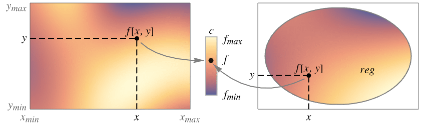
- この関数は,プロットされている領域上の x と y の値で f を評価し,色関数
を使って f[x,y]の各値を色にマッピングする. - プロットは集合
を可視化する.ただし,
は
の値を色にマッピングする色関数である. - f を評価しても実数にならない位置には,密度プロットの背景が見えるように穴が残される.
- DensityPlotは,実質的にBlockを使い変数 x と変数 y を局所的なものとして扱う.
- DensityPlotには属性HoldAllがあり,x と y に特定の数値を割り当てた後ではじめて f を評価する.
- 場合によっては,x と y に特定の数値が割り当てられる前にEvaluateを用いて f を記号的に評価した方が効率がよいことがある.
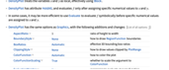
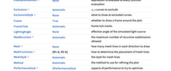
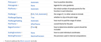
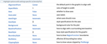
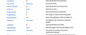
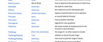
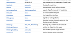
- DensityPlotは,Graphicsと同じオプションに,以下の追加・修正を加えたオプションを使用することができる. [全オプションのリスト]
- PlotLegendsのよく使われる設定
-
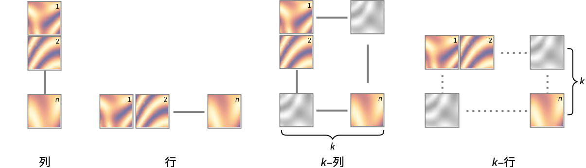
None 凡例は使わない Automatic ColorFunctionから凡例を自動的に決定する Placed[lspec,…] 凡例の置き方を指定する - 複数のプロットパネルのそれぞれで単一の密度を表示するPlotLayoutの可能な設定には以下がある.
-
"Column" パネルの列で異なる密度を使う "Row" パネルの行で異なる密度を使う {"Column",k},{"Row",k} k 列(行)を使う {"Column",UpTo[k]},{"Row",UpTo[k]} 最大で k 列(行)を使う - DensityPlotはまず,PlotPointsで指定された等間隔のサンプル点の格子で f を評価する.次に適応的アルゴリズムを用いて,滑らかな等高線を得るために最高MaxRecursion回まで再分割する.
- DensityPlotは有限個のサンプル点しか使わないので,関数の特徴を見付けられない可能性もあるので注意されたい.結果の検証にはPlotPointsとMaxRecursionの設定値を大きくしてみるとよい.
- Mesh->Allの設定では,DensityPlotは使用するすべての部分分割を表示するようにメッシュラインを描く.
- デフォルト設定のMeshFunctions->{#1&,#2&}では,x, y のメッシュが描かれる.
- MeshFunctions,RegionFunctionの関数に渡される引数は x,y,f である.
- ColorFunctionには,デフォルトで f のスケールされた値によって与えられた単一の引数が与えられる.
- デフォルト設定のExclusions->AutomaticとExclusionsStyle->Noneでは,DensityPlotが不連続曲線を検知すると,そこで表示される密度の連続性が途切れる.
- ScalingFunctionsの可能な設定値
-
sf f の値をスケールする {sx,sy} x 軸と y 軸をスケールする {sx,sy,sf} x 軸,y 軸,f の値をスケールする - 各スケーリング関数 siは,文字列"scale"または{g,g-1}である.g-1は g の逆数である.
- DensityPlotはGraphics[GraphicsComplex[data]]を返す.
全オプションのリスト
例題
すべて開く すべて閉じる例 (4)
DensityPlot[Sin[x]Sin[y], {x, -4, 4}, {y, -3, 3}]DensityPlot[Sin[x]Sin[y], {x, -4, 4}, {y, -3, 3}, ColorFunction -> "SunsetColors", PlotLegends -> Automatic]DensityPlot[Sin[x]Sin[y], {x, -4, 4}, {y, -3, 3}, ColorFunction -> "CMYKColors", PlotPoints -> 35, MeshFunctions -> {#3&, #3&}, Mesh -> {Range[-1, 1, 0.4], Range[-0.8, 0.8, 0.4]}, MeshStyle -> Opacity[0.5, Black]]DensityPlot[{Sin[x]Cos[y], Sin[x + y]Cos[x - y]}, {x, -5, 5}, {y, -5, 5}, PlotLayout -> "Row"]スコープ (19)
サンプリング (11)
関数が急激に変化するところではより多くの点がサンプルとして取られる:
DensityPlot[Sin[x y], {x, 0, 3}, {y, 0, 3}, Mesh -> All]DensityPlot[1 / (x ^ 2 + y ^ 2), {x, -1, 1}, {y, -1, 1}]DensityPlot[Sqrt[x y], {x, -1, 1}, {y, -1, 1}]DensityPlot[Im[Sqrt[(x + I y) ^ 3]], {x, -2, 2}, {y, -2, 2}]PlotPointsとMaxRecursionを使って適応的サンプリングを制御する:
Grid[Table[DensityPlot[Sin[x y], {x, 0, 4}, {y, 0, 4}, PlotPoints -> pp, MaxRecursion -> mr, Mesh -> None], {mr, {0, 2}}, {pp, {5, 15}}]]PlotRangeを使って関心領域に焦点を当てる:
{DensityPlot[x ^ 4 - 2x ^ 2 + y ^ 4 - 2y ^ 2 + 5, {x, -2, 2}, {y, -2, 2}], DensityPlot[x ^ 4 - 2x ^ 2 + y ^ 4 - 2y ^ 2 + 1, {x, -2, 2}, {y, -2, 2}, PlotRange -> {-2, 2}, ClippingStyle -> None]}Exclusionsを使って曲線を除いたり結果の曲面を分割したりする:
f = 1 / ChebyshevU[x y - 1, 2];{DensityPlot[f, {x, -5, 5}, {y, -5, 5}, ClippingStyle -> Automatic], DensityPlot[f, {x, -5, 5}, {y, -5, 5}, ClippingStyle -> Automatic, Exclusions -> {x == 0, y == 0}]}RegionFunctionを使って曲面を不等式で与えられる領域に限る:
DensityPlot[Sin[x + y ^ 2], {x, -3, 3}, {y, -2, 2}, RegionFunction -> Function[{x, y, z}, 0 < x + y ^ 2 < Pi]]DensityPlot[Sin[x + Cos[y]], {x, y}∈Disk[{0, 0}, 3]]領域はMeshRegionで指定することができる:
𝒟 = MeshRegion[{{0, 0}, {5, -2}, {3, 0}, {5, 2}}, Polygon[{1, 2, 3, 4}]];DensityPlot[Sin[x]Cos[y], {x, y}∈𝒟]DensityPlot[(x y^2/x^2 + y^4), {x, -Infinity, Infinity}, {y, -Infinity, Infinity}]プレゼンテーション (8)
DensityPlot[Sin[x y], {x, 0, 3}, {y, 0, 3}, FrameLabel -> {x, y}, PlotLabel -> Sin[x y], ColorFunction -> "SolarColors"]DensityPlot[Sin[x y], {x, 0, 3}, {y, 0, 3}, ColorFunction -> GrayLevel]DensityPlot[Sin[x y], {x, 0, 3}, {y, 0, 3}, ColorFunction -> "SouthwestColors", PlotPoints -> 35]DensityPlot[Sin[x y], {x, 0, 3}, {y, 0, 3}, ColorFunction -> "SouthwestColors", PlotPoints -> 35, PlotLegends -> Automatic]曲面用のインタラクティブなTooltipを用意する:
DensityPlot[Tooltip[Sqrt[x y]], {x, -2, 2}, {y, -2, 2}, ColorFunction -> "DeepSeaColors"]DensityPlot[Sin[x y], {x, 0, 3}, {y, 0, 3}, Mesh -> 5, ColorFunction -> "DarkRainbow", MeshStyle -> {Purple, Yellow}, PlotPoints -> 35]DensityPlot[Sin[x y], {x, 0, 3}, {y, 0, 3}, ColorFunction -> "TemperatureMap", PlotPoints -> 35, MeshFunctions -> {#3&, #3&}, Mesh -> {Range[-1, 1, 0.4], Range[-0.8, 0.8, 0.4]}, MeshStyle -> {Black, Dashed}]単純な目盛,コントラストのはっきりしたカラースキームというテーマを使う:
DensityPlot[Sin[x]Sin[y], {x, -4, 4}, {y, -3, 3}, PlotTheme -> "Marketing"]DensityPlot[{Sin[x]Cos[y], Sin[x + y]Cos[x - y]}, {x, -7, 7}, {y, -7, 7}, PlotLayout -> "Row"]DensityPlot[{Sin[x]Cos[y], Sin[x + y]Cos[x - y]}, {x, -7, 7}, {y, -7, 7}, PlotLayout -> "Column"]オプション (89)
AspectRatio (4)
デフォルトで,DensityPlotは縦横に同じ長さを使う:
DensityPlot[Sin[x]Cos[y], {x, -2Pi, 2Pi}, {y, -Pi / 2, 3Pi / 2}]DensityPlot[Sin[x]Cos[y], {x, -2Pi, 2Pi}, {y, -Pi / 2, 3Pi / 2}, AspectRatio -> 1 / 2]AspectRatioAutomaticはプロット範囲から比を決定する:
DensityPlot[Sin[x]Cos[y], {x, -2Pi, 2Pi}, {y, -Pi / 2, 3Pi / 2}, AspectRatio -> Automatic]AspectRatioFullは他の構造物の中にぴったり収まるように縦横の長さを調整する:
plot = DensityPlot[Sin[x]Cos[y], {x, -2Pi, 2Pi}, {y, -Pi / 2, 3Pi / 2}, AspectRatio -> Full];{Framed[Pane[plot, {50, 100}]], Framed[Pane[plot, {100, 100}]], Framed[Pane[plot, {100, 50}]]}Axes (4)
デフォルトで,DensityPlotは軸ではなく枠を使う:
DensityPlot[x Sin[y], {x, -5, 5}, {y, -5, 5}]DensityPlot[x Sin[y], {x, -5, 5}, {y, -5, 5}, Frame -> False, Axes -> True]AxesOriginを使って軸の交点を指定する:
DensityPlot[x Sin[y], {x, -5, 5}, {y, -5, 5}, Frame -> False, Axes -> True, AxesOrigin -> {1, 1}]{DensityPlot[x Sin[y], {x, -5, 5}, {y, -5, 5}, Frame -> False, Axes -> {True, False}], DensityPlot[x Sin[y], {x, -5, 5}, {y, -5, 5}, Frame -> False, Axes -> {False, True}]}AxesLabel (4)
DensityPlot[Sin[x ] + Cos[y], {x, -5, 5}, {y, -5, 5}, Frame -> False, Axes -> True]DensityPlot[Sin[x ] + Cos[y], {x, -5, 5}, {y, -5, 5}, Frame -> False, Axes -> True, AxesLabel -> y]DensityPlot[Sin[x ] + Cos[y], {x, -5, 5}, {y, -5, 5}, Frame -> False, Axes -> True, AxesLabel -> {"x-label", "y-label"}]DensityPlotで指定された変数に基づくラベルを使う:
DensityPlot[Sin[x ] + Cos[y], {x, -5, 5}, {y, -5, 5}, Frame -> False, Axes -> True, AxesLabel -> Automatic]AxesOrigin (2)
AxesStyle (4)
DensityPlot[x Sin[y], {x, -5, 5}, {y, -5, 5}, Frame -> False, Axes -> True, AxesStyle -> Red]DensityPlot[x Sin[y], {x, -5, 5}, {y, -5, 5}, Frame -> False, Axes -> True, AxesStyle -> {Red, Blue}]DensityPlot[x Sin[y], {x, -5, 5}, {y, -5, 5}, Frame -> False, Axes -> True, AxesStyle -> Green, TicksStyle -> Black]DensityPlot[x Sin[y], {x, -5, 5}, {y, -5, 5}, Frame -> False, Axes -> True, AxesStyle -> Green, LabelStyle -> Black]BoundaryStyle (3)
DensityPlot[Sin[x y], {x, -2, 2}, {y, -2, 2}, BoundaryStyle -> Red]BoundaryStyleはRegionFunctionで切り取られた領域に適用される:
DensityPlot[Sin[x y], {x, -2, 2}, {y, -2, 2}, BoundaryStyle -> Red, RegionFunction -> Function[{x, y, z}, x ^ 2 + y ^ 2 ≥ 1]]BoundaryStyleはExclusionsによって切り取られた部分には適用されない:
DensityPlot[Im[Sqrt[x + I y]], {x, -2, 2}, {y, -2, 2}, BoundaryStyle -> Red]代りにExclusionsStyleを使う:
DensityPlot[Im[Sqrt[x + I y]], {x, -2, 2}, {y, -2, 2}, ExclusionsStyle -> Red]ClippingStyle (4)
DensityPlot[Im[Gamma[x + I y]], {x, -3.5, 3.5}, {y, -3.5, 3.5}, ClippingStyle -> Automatic]DensityPlot[Im[Gamma[x + I y]], {x, -3.5, 3.5}, {y, -3.5, 3.5}, ClippingStyle -> None]DensityPlot[Im[Gamma[x + I y]], {x, -3.5, 3.5}, {y, -3.5, 3.5}, ClippingStyle -> Pink]切り取られた部分が上のところに薄い赤を,下のところにピンクを使う:
DensityPlot[Im[Gamma[x + I y]], {x, -3.5, 3.5}, {y, -3.5, 3.5}, ClippingStyle -> {Pink, LightRed}]ColorFunction (5)
DensityPlot[x + Sin[x ^ 2 + y ^ 2], {x, -4, 4}, {y, -4, 4}, ColorFunction -> Hue]DensityPlot[y + Sin[x ^ 2 + 3y], {x, -3, 3}, {y, -3, 3}, ColorFunction -> GrayLevel]DensityPlot[y + Sin[x ^ 2 + 3y], {x, -3, 3}, {y, -3, 3}, ColorFunction -> "SunsetColors"]DensityPlot[y + Sin[x ^ 2 + 3y], {x, -3, 3}, {y, -3, 3}, ColorFunction -> (Hue[2 / 5, 2 / 3, #]&)]DensityPlot[y + Sin[x ^ 2 + 3y], {x, -3, 3}, {y, -3, 3}, ColorFunction -> (RGBColor[1 - #, #, 1]&)]ColorFunctionScaling (1)
ColorFunctionScalingをFalseにして自然な値の範囲を得る:
DensityPlot[550 + 150 Sin[x]Sin[y], {x, 0, 2Pi}, {y, 0, 2Pi}, ColorFunction -> (ColorData["VisibleSpectrum"][#1]&), ColorFunctionScaling -> False, PlotPoints -> 50]EvaluationMonitor (2)
DensityPlotがどこで関数をサンプルするかを示す:
ListPlot[Reap[DensityPlot[Sin[x]Sin[y], {x, -2, 2}, {y, -3, 3}, EvaluationMonitor :> Sow[{x, y}]]][[-1, 1]]]Block[{k = 0}, DensityPlot[Sin[x y], {x, 0, 2}, {y, 0, 2}, EvaluationMonitor :> k++];k]Exclusions (6)
以下では除外するものを計算するのに自動メソッドが使われている:
DensityPlot[Im[ArcSin[x + I y]], {x, -2, 2}, {y, -2, 2}]DensityPlot[Im[ArcSin[x + I y]], {x, -2, 2}, {y, -2, 2}, Exclusions -> None]DensityPlot[ 1 / (y ^ 2 - x ^ 3 + 3x - 3), {x, -3, 3}, {y, -3, 3}, Exclusions -> {y ^ 2 - x ^ 3 + 3x - 3 == 0}, ClippingStyle -> Automatic]DensityPlot[Tan[x y] + 1 / (y ^ 2 - x ^ 3 + 3x - 3), {x, -2, 2}, {y, -2, 2}, Exclusions -> {Cos[x y] == 0, y ^ 2 - x ^ 3 + 3x - 3 == 0}, ClippingStyle -> Automatic]DensityPlot[Im[Sqrt[x + I y]], {x, -2, 2}, {y, -2, 2}, Exclusions -> {{y == 0, x ≤ 0}}]DensityPlot[Im[(x + I y) ^ (1 / 3)] / (x ^ 2 - y ^ 2), {x, -2, 2}, {y, -2, 2}, Exclusions -> {Automatic, x ^ 2 - y ^ 2 == 0}, Mesh -> False, ClippingStyle -> Automatic]//QuietExclusionsStyle (1)
ImageSize (7)
Tiny,Small,Medium,Largeのように名前付きのサイズを使う:
{DensityPlot[Sin[x]Sin[y], {x, -4, 4}, {y, -3, 3}, ImageSize -> Tiny], DensityPlot[Sin[x]Sin[y], {x, -4, 4}, {y, -3, 3}, ImageSize -> Small]}{DensityPlot[Sin[x]Sin[y], {x, -4, 4}, {y, -3, 3}, ImageSize -> 150], DensityPlot[Sin[x]Sin[y], {x, -4, 4}, {y, -3, 3}, AspectRatio -> 1.5, ImageSize -> 150]}{DensityPlot[Sin[x]Sin[y], {x, -4, 4}, {y, -3, 3}, ImageSize -> {Automatic, 150}], DensityPlot[Sin[x]Sin[y], {x, -4, 4}, {y, -3, 3}, AspectRatio -> 2, ImageSize -> {Automatic, 150}]}{DensityPlot[Sin[x]Sin[y], {x, -4, 4}, {y, -3, 3}, ImageSize -> UpTo[200]], DensityPlot[Sin[x]Sin[y], {x, -4, 4}, {y, -3, 3}, AspectRatio -> 2, ImageSize -> UpTo[200]]}グラフィックスの幅と高さを指定し,必要な場合は空白で充填する:
DensityPlot[Sin[x]Sin[y], {x, -4, 4}, {y, -3, 3}, ImageSize -> {300, 200}, Background -> StandardGray]AspectRatioFullとすると使用可能な空間が埋められる:
DensityPlot[Sin[x]Sin[y], {x, -4, 4}, {y, -3, 3}, AspectRatio -> Full, ImageSize -> {300, 200}, Background -> StandardGray]{DensityPlot[Sin[x]Sin[y], {x, -4, 4}, {y, -3, 3}, ImageSize -> {UpTo[150], UpTo[100]}], DensityPlot[Sin[x]Sin[y], {x, -4, 4}, {y, -3, 3}, AspectRatio -> 2, ImageSize -> {UpTo[150], UpTo[100]}]}ImageSizeFullを使ってオブジェクトの中の使用可能な空間を埋める:
Framed[Pane[DensityPlot[Sin[x]Sin[y], {x, -4, 4}, {y, -3, 3}, ImageSize -> Full, Background -> StandardGray], {200, 100}]]Framed[Pane[DensityPlot[Sin[x]Sin[y], {x, -4, 4}, {y, -3, 3}, AspectRatio -> Full, ImageSize -> {Scaled[0.5], Scaled[0.5]}, Background -> StandardGray], {200, 100}]]MaxRecursion (1)
Mesh (6)
DensityPlot[Sin[x + y ^ 2], {x, -3, 3}, {y, -2, 2}, Mesh -> None]{DensityPlot[Sin[x + y ^ 2], {x, -3, 3}, {y, -2, 2}, Mesh -> Full], DensityPlot[Sin[x + y ^ 2], {x, -3, 3}, {y, -2, 2}, Mesh -> All]}DensityPlot[Sin[x + y ^ 2], {x, -3, 3}, {y, -2, 2}, Mesh -> 5]
方向に3本のメッシュラインを,
方向に6本のメッシュラインを使う:
DensityPlot[Sin[x + y ^ 2], {x, -3, 3}, {y, -2, 2}, Mesh -> {3, 6}]DensityPlot[Sin[x + y ^ 2], {x, -3, 3}, {y, -2, 2}, Mesh -> {{-1}, {0}}]DensityPlot[Sin[x + y ^ 2], {x, -3, 3}, {y, -2, 2}, Mesh -> {{{-1, Red}}, {{0, Blue}}}]MeshFunctions (3)
DensityPlot[Sin[x + y ^ 2], {x, -3, 3}, {y, -2, 2}, MeshFunctions -> {#3&}, Mesh -> 5]DensityPlot[Sin[x + y ^ 2], {x, -3, 3}, {y, -2, 2}, MeshFunctions -> {#1&, #2&}, Mesh -> {5, 5}]DensityPlot[Sin[x + y ^ 2], {x, -3, 3}, {y, -2, 2}, MeshFunctions -> {Norm[{#1, #2, #3}]&}, Mesh -> 5]MeshStyle (2)
PerformanceGoal (2)
Timing[DensityPlot[Sin[x + y ^ 2], {x, -2, 2}, {y, -2, 2}, ColorFunction -> "Rainbow", PerformanceGoal -> "Quality"]]Timing[DensityPlot[Sin[x + y ^ 2], {x, -2, 2}, {y, -2, 2}, ColorFunction -> "Rainbow", PerformanceGoal -> "Speed"]]PlotLayout (3)
DensityPlot[{Cos[x], Cos[x + y], Cos[x + y ^ 2]}, {x, -3, 3}, {y, -2, 2}, ImageSize -> Medium, PlotLayout -> "Column"]DensityPlot[{Cos[x], Cos[x + y], Cos[x + y ^ 2]}, {x, -3, 3}, {y, -2, 2}, ImageSize -> Medium, PlotLayout -> "Row"]DensityPlot[{Cos[x], Cos[x + y], Cos[x + y ^ 2]}, {x, -3, 3}, {y, -2, 2}, ImageSize -> Medium, PlotLayout -> {"Column", 2}]DensityPlot[{Sin[x + y], Sin[2 x + y], Sin[3 x + y], Sin[4 x + y], Sin[5 x + y], Sin[6 x + y]}, {x, -3, 3}, {y, -2, 2}, ImageSize -> Medium, PlotLayout -> {"Column", UpTo[4]}]DensityPlot[{Sin[x + y], Sin[2 x + y], Sin[3 x + y], Sin[4 x + y], Sin[5 x + y], Sin[6 x + y]}, {x, -3, 3}, {y, -2, 2}, ImageSize -> Medium, PlotLayout -> {"Column", 4}]PlotLegends (4)
DensityPlot[Sin[2 x + y]Cos[x - 2y], {x, 0, Pi}, {y, 0, Pi}, PlotLegends -> Automatic]PlotLegendsは自動的に色関数にマッチする:
DensityPlot[Sin[2 x + y]Cos[x - 2y], {x, 0, Pi}, {y, 0, Pi}, ColorFunction -> "GrayYellowTones", PlotLegends -> Automatic]Placedを使って凡例の位置を変える:
Table[DensityPlot[Sin[x + y ^ 2], {x, -3, 3}, {y, -2, 2}, PlotLegends -> Placed[Automatic, pos], PlotLabel -> pos, ImageSize -> 150], {pos, {Before, After, Above, Below}}]BarLegendを使って凡例の外観を変える:
DensityPlot[Sin[x + y ^ 2], {x, -3, 3}, {y, -2, 2}, PlotLegends -> BarLegend[Automatic, LegendMarkerSize -> 180, LegendFunction -> "Frame", LegendMargins -> 5, LegendLabel -> "z-value"]]PlotPoints (2)
Table[DensityPlot[Sin[x + y ^ 2], {x, -3, 3}, {y, -2, 2}, Mesh -> None, MaxRecursion -> 0, PlotPoints -> pp], {pp, {5, 10, 15, 20}}]DensityPlot[Sin[2x]y, {x, 0, 2Pi}, {y, -1, 1}, PlotPoints -> {20, 5}, Mesh -> Full]PlotRange (4)
DensityPlot[1 / (x ^ 2 + y ^ 2), {x, -2, 2}, {y, -2, 2}]DensityPlot[1 / (x ^ 2 + y ^ 2), {x, -2, 2}, {y, -2, 2}, PlotRange -> All]DensityPlot[Sqrt[1 - x ^ 2 - y ^ 2], {x, -2, 2}, {y, -2, 2}, PlotRange -> Full]DensityPlot[Sqrt[1 - x ^ 2 - y ^ 2], {x, -2, 2}, {y, -2, 2}, PlotRange -> Automatic]{DensityPlot[x ^ 2 - y ^ 2, {x, -4, 4}, {y, -4, 4}], DensityPlot[x ^ 2 - y ^ 2, {x, -4, 4}, {y, -4, 4}, PlotRange -> {-2, 2}]}PlotTheme (1)
RegionFunction (3)
DensityPlot[Sin[x + y ^ 2], {x, -2, 2}, {y, -2, 2}, RegionFunction -> Function[{x, y, z}, 2 < x ^ 2 + y ^ 2 < 5], BoundaryStyle -> Red]DensityPlot[Sin[x + y ^ 2], {x, -2, 2}, {y, -2, 2}, RegionFunction -> Function[{x, y, z}, 0 < Mod[x ^ 2 + y ^ 2, 2] < 1], BoundaryStyle -> Red]DensityPlot[Sin[x + y ^ 2], {x, -2, 2}, {y, -2, 2}, RegionFunction -> Function[{x, y, z}, (x - 1 / 2) ^ 2 + y ^ 2 > 1 && (x + 1 / 2) ^ 2 + y ^ 2 > 1], BoundaryStyle -> Red]ScalingFunctions (9)
DensityPlot[Max[x, y], {x, 0, 10}, {y, 0, 10}, Exclusions -> None]DensityPlot[Max[x, y], {x, 0, 10}, {y, 0, 10}, ScalingFunctions -> {None, "Log"}, Exclusions -> None]DensityPlot[Max[x, y], {x, 0, 10}, {y, 0, 10}, ScalingFunctions -> {None, "Reverse"}, Exclusions -> None]DensityPlot[Max[x, y], {x, 0, 10}, {y, 0, 10}, ScalingFunctions -> {None, "Reciprocal"}, PlotRangePadding -> None, Exclusions -> None]DensityPlot[Max[x, y], {x, 0, 10}, {y, 0, 10}, ScalingFunctions -> {"Reverse", "Log"}, Exclusions -> None]DensityPlot[Max[x, y], {x, 0, 10}, {y, 0, 10}, ScalingFunctions -> {"Reverse", None}, Exclusions -> None]DensityPlot[Max[x, y], {x, 0, 10}, {y, 0, 10}, ScalingFunctions -> {None, {-Log[#]&, Exp[-#]&}}, Exclusions -> None]TicksとGridLinesの中の位置は自動的にスケールされる:
DensityPlot[Sin[x + y ^ 2], {x, 0.1, 2}, {y, -2, 2}, RegionFunction -> Function[{x, y, z}, 2 < x ^ 2 + y ^ 2 < 5], ScalingFunctions -> {"Log", None}, FrameTicks -> {{Automatic, Automatic}, {2 ^ Range[-5, 2], Automatic}}, GridLines -> All]PlotRangeは自動的にスケールされる:
DensityPlot[x ^ 2 + y ^ 2, {x, 0, 10}, {y, 0, 10}, ScalingFunctions -> {None, "Log"}, PlotRange -> {1, 100}]アプリケーション (7)
DensityPlot[Evaluate[Sum[Sin[RandomReal[5, 2].{x, y}], {5}]], {x, 0, 5}, {y, 0, 5}, ColorFunction -> "Rainbow", PlotPoints -> 50]NDSolve[{D[u[t, x], t] == D[u[t, x], x, x], u[0, x] == 0, u[t, 0] == Sin[t], u[t, 5] == 0}, u, {t, 0, 10}, {x, 0, 5}]DensityPlot[Evaluate[u[t, x] /. %], {t, 0, 10}, {x, 0, 5}, PlotRange -> All, ColorFunction -> "SunsetColors"]鞍型曲面をプロットする.メッシュ曲線は関数が零のところを示している:
DensityPlot[y ^ 2 - x ^ 2, {x, -4, 4}, {y, -4, 4}, MeshFunctions -> {#3&}, MeshStyle -> Directive[Dashed, Thickness[Medium]], Mesh -> {{0}}, PlotRange -> {-4, 4}, ClippingStyle -> Automatic]1/2,1,3/2に等ノルムのメッシュラインが入った1, 2, 3および
ノルム:
Table[DensityPlot[Norm[{x, y}, p], {x, -1.5, 1.5}, {y, -1.5, 1.5}, Ticks -> None, MeshFunctions -> {#3&}, Mesh -> {{1 / 2, 1, 3 / 2}}, MeshStyle -> Directive[Dashed, GrayLevel[0.3]], Exclusions -> None], {p, {1, 2, 3, Infinity}}]Table[DensityPlot[Arg[f[x + I y]], {x, -2Pi, 2Pi}, {y, -2, 2}, ColorFunction -> "SunsetColors", FrameTicks -> {Range[-2Pi, 2Pi, Pi], Automatic, None, None}], {f, {Sin, Cos, Tan, Cot}}]Table[DensityPlot[f[ArcSin[(x + I y) ^ 2]], {x, -2, 2}, {y, -2, 2}, ColorFunction -> "DarkRainbow", ExclusionsStyle -> Red], {f, {Re, Im, Abs, Arg}}]DensityPlot[(x - 1) ^ 2 + 100(x ^ 2 - y) ^ 2, {x, -2, 2}, {y, -2, 2}, ClippingStyle -> Automatic, ColorFunction -> "Rainbow", PlotPoints -> 30]DensityPlot[Log[(x - 1) ^ 2 + 100(x ^ 2 - y) ^ 2], {x, -2, 2}, {y, -2, 2}, ClippingStyle -> Automatic, ColorFunction -> "Rainbow", PlotPoints -> 30]特性と関係 (9)
DensityPlotは,必要な場合はより多くの点をサンプルとして取る:
DensityPlot[Sin[x y], {x, 0, 3}, {y, 0, 3}, Mesh -> All]ContourPlotを使って分割された等曲線と等高線の領域を得る:
ContourPlot[Sin[x y], {x, 0, 3}, {y, 0, 3}]連続データのプロットにListDensityPlotを使う:
data = Table[Sin[x y], {x, 0, 3, .1}, {y, 0, 3, .1}];ListDensityPlot[data]Plot3Dを使って三次元曲面を得る:
Plot3D[Sin[x y], {x, 0, 3}, {y, 0, 3}]ColorFunctionを加えてオーバーレイ密度を得る:
Plot3D[Sin[x y], {x, 0, 3}, {y, 0, 3}, ColorFunction -> "SunsetColors", Mesh -> None]ComplexPlotは,大きさによる色と陰影を使って関数の位相をプロットする:
ComplexPlot[Sin[z] ^ 3 / (z + 1) ^ 4, {z, -5 - 5I, 5 + 5I}]DensityPlot[Arg[Sin[x + I * y] ^ 3 / (x + I * y + 1) ^ 4], {x, -5, 5}, {y, -5, 5}]ArrayPlotまたはMatrixPlotを離散データに使う:
ArrayPlot[CellularAutomaton[30, {{1}, 0}, 30]]MatrixPlot[Last@SchurDecomposition@RandomReal[1, {50, 50}]]Plotを一変量関数に使う:
Plot[Sin[x] + Sin[Sqrt[2]x], {x, 0, 20}]ParametricPlotを平面のパラメトリック曲線と領域に使う:
{ParametricPlot[{Cos[θ], Sin[θ]}, {θ, 0, 2Pi}], ParametricPlot[{r Cos[θ], r Sin[θ]}, {θ, 0, 2Pi}, {r, 1 / 2, 1}]}ContourPlot3DとRegionPlot3Dを陰的な曲面と領域に使う:
{ContourPlot3D[Sin[x y] == z, {x, -2, 2}, {y, -2, 2}, {z, -2, 2}],
RegionPlot3D[Sin[x y] ≥ z, {x, -2, 2}, {y, -2, 2}, {z, -2, 2}]}考えられる問題 (2)
分割の色関数または区分色関数を使うと,色の変わり目の境界線がはっきりしなくなることがある:
DensityPlot[Sin[y]Sin[y - x], {x, 0, 4Pi}, {y, 0, 4Pi}, ColorFunction -> (If[# > 0, Blue, White]&), ColorFunctionScaling -> False, PlotPoints -> 50]分割問題に,ContourPlotを代りに使う:
ContourPlot[Sin[y]Sin[y - x], {x, 0, 4Pi}, {y, 0, 4Pi}, Contours -> {0}, ContourShading -> {White, Blue}]急激に変化する色関数あるいは色密度は副作用を示すことがある:
DensityPlot[Sin[x y], {x, 0, 4}, {y, 0, 4}, ColorFunction -> Hue]PlotPointsを使ってサンプル密度を高くする:
DensityPlot[Sin[x y], {x, 0, 4}, {y, 0, 4}, ColorFunction -> Hue, PlotPoints -> 100]おもしろい例題 (2)
$InverseTrigFunctions = {ArcSin, ArcCos, ArcSec, ArcCsc, ArcTan, ArcCot, ArcSinh, ArcCosh, ArcSech, ArcCsch, ArcTanh, ArcCoth};Table[DensityPlot[Im[f[(x + I y) ^ 3]], {x, -2, 2}, {y, -2, 2}, ColorFunction -> "Pastel", ExclusionsStyle -> {None, Purple}, Mesh -> None, PlotLabel -> Im[f[(x + I y) ^ 3]], Ticks -> None], {f, $InverseTrigFunctions}]$TrigFunctions = {Sin, Cos, Sec, Csc, Tan, Cot, ArcSin, ArcCos, ArcSec, ArcCsc, ArcTan, ArcCot, Sinh, Cosh, Sech, Csch, Tanh, Coth, ArcSinh, ArcCosh, ArcSech, ArcCsch, ArcTanh, ArcCoth};Table[DensityPlot[Abs[f[x + I y]], {x, -2, 2}, {y, -2, 2}, MeshFunctions -> Function@@@{{{x, y, z}, Re[f[x + I y]]}, {{x, y, z}, Im[f[x + I y]]}}, MeshStyle -> {Opacity[1 / 3], Opacity[2 / 3]}, ColorFunction -> "NeonColors", PlotLabel -> f, Ticks -> None, Mesh -> 10], {f, $TrigFunctions}]テクニカルノート
履歴
1988 で導入 (1.0) | 2007 で更新 (6.0) ▪ 2008 (7.0) ▪ 2012 (9.0) ▪ 2014 (10.0) ▪ 2017 (11.1) ▪ 2021 (13.0)
テキスト
Wolfram Research (1988), DensityPlot, Wolfram言語関数, https://reference.wolfram.com/language/ref/DensityPlot.html (2021年に更新).
CMS
Wolfram Language. 1988. "DensityPlot." Wolfram Language & System Documentation Center. Wolfram Research. Last Modified 2021. https://reference.wolfram.com/language/ref/DensityPlot.html.
APA
Wolfram Language. (1988). DensityPlot. Wolfram Language & System Documentation Center. Retrieved from https://reference.wolfram.com/language/ref/DensityPlot.html
BibTeX
@misc{reference.wolfram_2026_densityplot, author="Wolfram Research", title="{DensityPlot}", year="2021", howpublished="\url{https://reference.wolfram.com/language/ref/DensityPlot.html}", note=[Accessed: 10-September-2026]}
BibLaTeX
@online{reference.wolfram_2026_densityplot, organization={Wolfram Research}, title={DensityPlot}, year={2021}, url={https://reference.wolfram.com/language/ref/DensityPlot.html}, note=[Accessed: 10-September-2026]}