DensityPlot[f,{x,xmin,xmax},{y,ymin,ymax}]
绘制关于 x 和 y 的函数 f 的密度图.
DensityPlot[f,{x,y}∈reg]
令变量 {x,y} 在几何区域 reg 中.
DensityPlot
DensityPlot[f,{x,xmin,xmax},{y,ymin,ymax}]
绘制关于 x 和 y 的函数 f 的密度图.
DensityPlot[f,{x,y}∈reg]
令变量 {x,y} 在几何区域 reg 中.
更多信息和选项
- DensityPlot 亦称为热图.
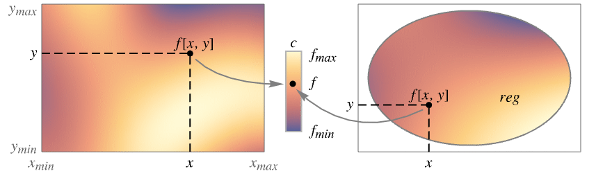
- 该函数在被绘制的域中的 x 和 y 值上计算 f,并使用一个颜色函数
将每个值 f[x,y] 映射到一个颜色上. - 该图将
这组数据可视化,其中
是一个将
值映射为颜色的颜色函数. - 在 f 无法计算得到实数的位置,密度图的背景处留有以“洞” (hole) 表示的记号.
- DensityPlot 实际上用 Block 把 x 和 y 当作本地数值.
- DensityPlot 的属性 HoldAll 决定仅在指定数值 x 和 y 后计算 f.
- 在某些情况下指定 x 和 y 之前用 Evaluate 计算 f 会更有效.
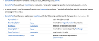
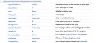
- DensityPlot 有和 Graphics 相同的选项,并有下列增加和变化: [所有选项的列表]
-
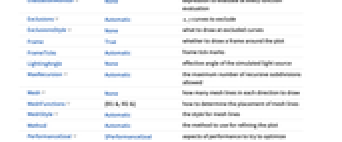
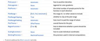
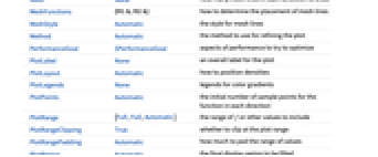
AspectRatio 1 长与宽的比例 BoundaryStyle None 如何绘制 RegionFunction 的边界 BoxRatios Automatic 3D 边框的长宽比例 ClippingStyle None 如何绘制 PlotRange 中的值 ColorFunction Automatic 如何对图着色 ColorFunctionScaling True 是否对 ColorFunction 的参数着色 EvaluationMonitor None 在每次函数计算时计算的表达式 Exclusions Automatic 不包含 x, y 的曲线 ExclusionsStyle None 需要绘制的除曲线外的内容 Frame True 是否绘制边框 FrameTicks Automatic 边框刻度 LightingAngle None 模拟光源的角度 MaxRecursion Automatic 纯量场的递归最大次数 Mesh None 背景网格线的数量 MeshFunctions {#1&,#2&} 决定网格线的位置 MeshStyle Automatic 网格线的风格 Method Automatic 绘图使用的方法 PerformanceGoal $PerformanceGoal 优化的目标 PlotLayout Automatic 如何定位密度 PlotLegends None 颜色梯度的图例 PlotPoints Automatic 函数在不同方向上样本点的初始值 PlotRange {Full,Full,Automatic} f 或其它值的范围 PlotRangeClipping True 是否锁定绘制范围 PlotRangePadding Automatic 垫衬多少值的范围 PlotTheme $PlotTheme 图形的全局主题 RegionFunction (True&) 决定是否包含一个点的方法 ScalingFunctions None 如何调整单独坐标 WorkingPrecision MachinePrecision 内部计算的精度 - PlotLegends 的典型设置包括:
-
None 不使用图例 Automatic 自动从 ColorFunction 确定图例 Placed[lspec,…] 指定图例位置 - 在多个绘图面板中显示单个密度的 PlotLayout 的可能设置包括:
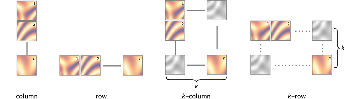
-
"Column" 在一列面板中使用不同的密度 "Row" 在一行面板中使用不同的密度 {"Column",k},{"Row",k} 使用 k 列或行 {"Column",UpTo[k]},{"Row",UpTo[k]} 使用至多 k 列或行 - DensityPlot 在由 PlotPoints 指定的等距离样本点组成的网格处对 f 进行初始计算. 之后使用一个自适应算法来进行至多 MaxRecursion 次细分,以生成平滑等高线.
- 由于 DensityPlot 仅使用有限的样本点,所以可能会丢失函数的特征. 可以尝试增加 PlotPoints 和 MaxRecursion 的设置来检验结果.
- 设置为 Mesh->All,DensityPlot 绘制网格线以显示所用的所有细分.
- 缺省设置 MeshFunctions->{#1&,#2&} 绘制 x、y 网格.
- 提供给函数 MeshFunctions 和 RegionFunction 的参数为 x、y、f.
- ColorFunction 可以只有一个缺省来自 f 的参数.
- 默认设置 Exclusions->Automatic 和 ExclusionsStyle->None 下,DensityPlot 在密度图找到的不连续曲线处打破连续性.
- ScalingFunctions 的可能设置包括:
-
sf 缩放 f 值 {sx,sy} 缩放 x 和 y 轴 {sx,sy,sf} 缩放 x 和 y 轴和 f 值 - 每个缩放函数 si 不是字符串 "scale" 就是 {g,g-1},其中 g-1 是 g 的反函数.
- DensityPlot 返回 Graphics[GraphicsComplex[data]].
所有选项的列表
范例
打开所有单元 关闭所有单元基本范例 (4)
DensityPlot[Sin[x]Sin[y], {x, -4, 4}, {y, -3, 3}]DensityPlot[Sin[x]Sin[y], {x, -4, 4}, {y, -3, 3}, ColorFunction -> "SunsetColors", PlotLegends -> Automatic]DensityPlot[Sin[x]Sin[y], {x, -4, 4}, {y, -3, 3}, ColorFunction -> "CMYKColors", PlotPoints -> 35, MeshFunctions -> {#3&, #3&}, Mesh -> {Range[-1, 1, 0.4], Range[-0.8, 0.8, 0.4]}, MeshStyle -> Opacity[0.5, Black]]DensityPlot[{Sin[x]Cos[y], Sin[x + y]Cos[x - y]}, {x, -5, 5}, {y, -5, 5}, PlotLayout -> "Row"]范围 (19)
Sampling (11)
DensityPlot[Sin[x y], {x, 0, 3}, {y, 0, 3}, Mesh -> All]DensityPlot[1 / (x ^ 2 + y ^ 2), {x, -1, 1}, {y, -1, 1}]DensityPlot[Sqrt[x y], {x, -1, 1}, {y, -1, 1}]DensityPlot[Im[Sqrt[(x + I y) ^ 3]], {x, -2, 2}, {y, -2, 2}]用 PlotPoints 和 MaxRecursion 来控制自适应采样:
Grid[Table[DensityPlot[Sin[x y], {x, 0, 4}, {y, 0, 4}, PlotPoints -> pp, MaxRecursion -> mr, Mesh -> None], {mr, {0, 2}}, {pp, {5, 15}}]]用 PlotRange 聚焦感兴趣的区域:
{DensityPlot[x ^ 4 - 2x ^ 2 + y ^ 4 - 2y ^ 2 + 5, {x, -2, 2}, {y, -2, 2}], DensityPlot[x ^ 4 - 2x ^ 2 + y ^ 4 - 2y ^ 2 + 1, {x, -2, 2}, {y, -2, 2}, PlotRange -> {-2, 2}, ClippingStyle -> None]}用 Exclusions 删除曲线或切割所得的曲面:
f = 1 / ChebyshevU[x y - 1, 2];{DensityPlot[f, {x, -5, 5}, {y, -5, 5}, ClippingStyle -> Automatic], DensityPlot[f, {x, -5, 5}, {y, -5, 5}, ClippingStyle -> Automatic, Exclusions -> {x == 0, y == 0}]}用 RegionFunction 将表面限定在由不等式给出的区域:
DensityPlot[Sin[x + y ^ 2], {x, -3, 3}, {y, -2, 2}, RegionFunction -> Function[{x, y, z}, 0 < x + y ^ 2 < Pi]]DensityPlot[Sin[x + Cos[y]], {x, y}∈Disk[{0, 0}, 3]]定义域可以由 MeshRegion 指定:
𝒟 = MeshRegion[{{0, 0}, {5, -2}, {3, 0}, {5, 2}}, Polygon[{1, 2, 3, 4}]];DensityPlot[Sin[x]Cos[y], {x, y}∈𝒟]DensityPlot[(x y^2/x^2 + y^4), {x, -Infinity, Infinity}, {y, -Infinity, Infinity}]Presentation (8)
DensityPlot[Sin[x y], {x, 0, 3}, {y, 0, 3}, FrameLabel -> {x, y}, PlotLabel -> Sin[x y], ColorFunction -> "SolarColors"]DensityPlot[Sin[x y], {x, 0, 3}, {y, 0, 3}, ColorFunction -> GrayLevel]DensityPlot[Sin[x y], {x, 0, 3}, {y, 0, 3}, ColorFunction -> "SouthwestColors", PlotPoints -> 35]DensityPlot[Sin[x y], {x, 0, 3}, {y, 0, 3}, ColorFunction -> "SouthwestColors", PlotPoints -> 35, PlotLegends -> Automatic]为表面提供交互式 Tooltip:
DensityPlot[Tooltip[Sqrt[x y]], {x, -2, 2}, {y, -2, 2}, ColorFunction -> "DeepSeaColors"]DensityPlot[Sin[x y], {x, 0, 3}, {y, 0, 3}, Mesh -> 5, ColorFunction -> "DarkRainbow", MeshStyle -> {Purple, Yellow}, PlotPoints -> 35]DensityPlot[Sin[x y], {x, 0, 3}, {y, 0, 3}, ColorFunction -> "TemperatureMap", PlotPoints -> 35, MeshFunctions -> {#3&, #3&}, Mesh -> {Range[-1, 1, 0.4], Range[-0.8, 0.8, 0.4]}, MeshStyle -> {Black, Dashed}]DensityPlot[Sin[x]Sin[y], {x, -4, 4}, {y, -3, 3}, PlotTheme -> "Marketing"]DensityPlot[{Sin[x]Cos[y], Sin[x + y]Cos[x - y]}, {x, -7, 7}, {y, -7, 7}, PlotLayout -> "Row"]DensityPlot[{Sin[x]Cos[y], Sin[x + y]Cos[x - y]}, {x, -7, 7}, {y, -7, 7}, PlotLayout -> "Column"]选项 (89)
AspectRatio (4)
默认情况下,DensityPlot 使用相同的宽度和高度:
DensityPlot[Sin[x]Cos[y], {x, -2Pi, 2Pi}, {y, -Pi / 2, 3Pi / 2}]DensityPlot[Sin[x]Cos[y], {x, -2Pi, 2Pi}, {y, -Pi / 2, 3Pi / 2}, AspectRatio -> 1 / 2]AspectRatioAutomatic 根据绘图范围确定比率:
DensityPlot[Sin[x]Cos[y], {x, -2Pi, 2Pi}, {y, -Pi / 2, 3Pi / 2}, AspectRatio -> Automatic]AspectRatioFull 调整高度和宽度以紧密适应其他结构内部:
plot = DensityPlot[Sin[x]Cos[y], {x, -2Pi, 2Pi}, {y, -Pi / 2, 3Pi / 2}, AspectRatio -> Full];{Framed[Pane[plot, {50, 100}]], Framed[Pane[plot, {100, 100}]], Framed[Pane[plot, {100, 50}]]}Axes (4)
默认情况下,DensityPlot 使用边框而不是轴:
DensityPlot[x Sin[y], {x, -5, 5}, {y, -5, 5}]DensityPlot[x Sin[y], {x, -5, 5}, {y, -5, 5}, Frame -> False, Axes -> True]使用 AxesOrigin 指定轴相交的位置:
DensityPlot[x Sin[y], {x, -5, 5}, {y, -5, 5}, Frame -> False, Axes -> True, AxesOrigin -> {1, 1}]{DensityPlot[x Sin[y], {x, -5, 5}, {y, -5, 5}, Frame -> False, Axes -> {True, False}], DensityPlot[x Sin[y], {x, -5, 5}, {y, -5, 5}, Frame -> False, Axes -> {False, True}]}AxesLabel (4)
DensityPlot[Sin[x ] + Cos[y], {x, -5, 5}, {y, -5, 5}, Frame -> False, Axes -> True]DensityPlot[Sin[x ] + Cos[y], {x, -5, 5}, {y, -5, 5}, Frame -> False, Axes -> True, AxesLabel -> y]DensityPlot[Sin[x ] + Cos[y], {x, -5, 5}, {y, -5, 5}, Frame -> False, Axes -> True, AxesLabel -> {"x-label", "y-label"}]根据 DensityPlot 中指定的变量使用标签:
DensityPlot[Sin[x ] + Cos[y], {x, -5, 5}, {y, -5, 5}, Frame -> False, Axes -> True, AxesLabel -> Automatic]AxesOrigin (2)
AxesStyle (4)
DensityPlot[x Sin[y], {x, -5, 5}, {y, -5, 5}, Frame -> False, Axes -> True, AxesStyle -> Red]DensityPlot[x Sin[y], {x, -5, 5}, {y, -5, 5}, Frame -> False, Axes -> True, AxesStyle -> {Red, Blue}]DensityPlot[x Sin[y], {x, -5, 5}, {y, -5, 5}, Frame -> False, Axes -> True, AxesStyle -> Green, TicksStyle -> Black]DensityPlot[x Sin[y], {x, -5, 5}, {y, -5, 5}, Frame -> False, Axes -> True, AxesStyle -> Green, LabelStyle -> Black]BoundaryStyle (3)
DensityPlot[Sin[x y], {x, -2, 2}, {y, -2, 2}, BoundaryStyle -> Red]BoundaryStyle 可使用 RegionFunction 切割的区域:
DensityPlot[Sin[x y], {x, -2, 2}, {y, -2, 2}, BoundaryStyle -> Red, RegionFunction -> Function[{x, y, z}, x ^ 2 + y ^ 2 ≥ 1]]BoundaryStyle 不支持 Exclusions 切割的区域:
DensityPlot[Im[Sqrt[x + I y]], {x, -2, 2}, {y, -2, 2}, BoundaryStyle -> Red]使用 ExclusionsStyle 代替:
DensityPlot[Im[Sqrt[x + I y]], {x, -2, 2}, {y, -2, 2}, ExclusionsStyle -> Red]ClippingStyle (4)
DensityPlot[Im[Gamma[x + I y]], {x, -3.5, 3.5}, {y, -3.5, 3.5}, ClippingStyle -> Automatic]DensityPlot[Im[Gamma[x + I y]], {x, -3.5, 3.5}, {y, -3.5, 3.5}, ClippingStyle -> None]DensityPlot[Im[Gamma[x + I y]], {x, -3.5, 3.5}, {y, -3.5, 3.5}, ClippingStyle -> Pink]DensityPlot[Im[Gamma[x + I y]], {x, -3.5, 3.5}, {y, -3.5, 3.5}, ClippingStyle -> {Pink, LightRed}]ColorFunction (5)
DensityPlot[x + Sin[x ^ 2 + y ^ 2], {x, -4, 4}, {y, -4, 4}, ColorFunction -> Hue]DensityPlot[y + Sin[x ^ 2 + 3y], {x, -3, 3}, {y, -3, 3}, ColorFunction -> GrayLevel]DensityPlot[y + Sin[x ^ 2 + 3y], {x, -3, 3}, {y, -3, 3}, ColorFunction -> "SunsetColors"]DensityPlot[y + Sin[x ^ 2 + 3y], {x, -3, 3}, {y, -3, 3}, ColorFunction -> (Hue[2 / 5, 2 / 3, #]&)]DensityPlot[y + Sin[x ^ 2 + 3y], {x, -3, 3}, {y, -3, 3}, ColorFunction -> (RGBColor[1 - #, #, 1]&)]ColorFunctionScaling (1)
设置 ColorFunctionScaling 为 False 得到值的自然范围:
DensityPlot[550 + 150 Sin[x]Sin[y], {x, 0, 2Pi}, {y, 0, 2Pi}, ColorFunction -> (ColorData["VisibleSpectrum"][#1]&), ColorFunctionScaling -> False, PlotPoints -> 50]EvaluationMonitor (2)
显示 DensityPlot 的对函数取样区域:
ListPlot[Reap[DensityPlot[Sin[x]Sin[y], {x, -2, 2}, {y, -3, 3}, EvaluationMonitor :> Sow[{x, y}]]][[-1, 1]]]Block[{k = 0}, DensityPlot[Sin[x y], {x, 0, 2}, {y, 0, 2}, EvaluationMonitor :> k++];k]Exclusions (6)
DensityPlot[Im[ArcSin[x + I y]], {x, -2, 2}, {y, -2, 2}]DensityPlot[Im[ArcSin[x + I y]], {x, -2, 2}, {y, -2, 2}, Exclusions -> None]DensityPlot[ 1 / (y ^ 2 - x ^ 3 + 3x - 3), {x, -3, 3}, {y, -3, 3}, Exclusions -> {y ^ 2 - x ^ 3 + 3x - 3 == 0}, ClippingStyle -> Automatic]DensityPlot[Tan[x y] + 1 / (y ^ 2 - x ^ 3 + 3x - 3), {x, -2, 2}, {y, -2, 2}, Exclusions -> {Cos[x y] == 0, y ^ 2 - x ^ 3 + 3x - 3 == 0}, ClippingStyle -> Automatic]DensityPlot[Im[Sqrt[x + I y]], {x, -2, 2}, {y, -2, 2}, Exclusions -> {{y == 0, x ≤ 0}}]DensityPlot[Im[(x + I y) ^ (1 / 3)] / (x ^ 2 - y ^ 2), {x, -2, 2}, {y, -2, 2}, Exclusions -> {Automatic, x ^ 2 - y ^ 2 == 0}, Mesh -> False, ClippingStyle -> Automatic]//QuietExclusionsStyle (1)
ImageSize (7)
使用有名称的尺寸,如 Tiny、Small、Medium 和 Large:
{DensityPlot[Sin[x]Sin[y], {x, -4, 4}, {y, -3, 3}, ImageSize -> Tiny], DensityPlot[Sin[x]Sin[y], {x, -4, 4}, {y, -3, 3}, ImageSize -> Small]}{DensityPlot[Sin[x]Sin[y], {x, -4, 4}, {y, -3, 3}, ImageSize -> 150], DensityPlot[Sin[x]Sin[y], {x, -4, 4}, {y, -3, 3}, AspectRatio -> 1.5, ImageSize -> 150]}{DensityPlot[Sin[x]Sin[y], {x, -4, 4}, {y, -3, 3}, ImageSize -> {Automatic, 150}], DensityPlot[Sin[x]Sin[y], {x, -4, 4}, {y, -3, 3}, AspectRatio -> 2, ImageSize -> {Automatic, 150}]}{DensityPlot[Sin[x]Sin[y], {x, -4, 4}, {y, -3, 3}, ImageSize -> UpTo[200]], DensityPlot[Sin[x]Sin[y], {x, -4, 4}, {y, -3, 3}, AspectRatio -> 2, ImageSize -> UpTo[200]]}DensityPlot[Sin[x]Sin[y], {x, -4, 4}, {y, -3, 3}, ImageSize -> {300, 200}, Background -> StandardGray]设置 AspectRatioFull 会填充可用空间:
DensityPlot[Sin[x]Sin[y], {x, -4, 4}, {y, -3, 3}, AspectRatio -> Full, ImageSize -> {300, 200}, Background -> StandardGray]{DensityPlot[Sin[x]Sin[y], {x, -4, 4}, {y, -3, 3}, ImageSize -> {UpTo[150], UpTo[100]}], DensityPlot[Sin[x]Sin[y], {x, -4, 4}, {y, -3, 3}, AspectRatio -> 2, ImageSize -> {UpTo[150], UpTo[100]}]}设置 ImageSizeFull 可填充对象内的可用空间:
Framed[Pane[DensityPlot[Sin[x]Sin[y], {x, -4, 4}, {y, -3, 3}, ImageSize -> Full, Background -> StandardGray], {200, 100}]]Framed[Pane[DensityPlot[Sin[x]Sin[y], {x, -4, 4}, {y, -3, 3}, AspectRatio -> Full, ImageSize -> {Scaled[0.5], Scaled[0.5]}, Background -> StandardGray], {200, 100}]]MaxRecursion (1)
Mesh (6)
DensityPlot[Sin[x + y ^ 2], {x, -3, 3}, {y, -2, 2}, Mesh -> None]{DensityPlot[Sin[x + y ^ 2], {x, -3, 3}, {y, -2, 2}, Mesh -> Full], DensityPlot[Sin[x + y ^ 2], {x, -3, 3}, {y, -2, 2}, Mesh -> All]}DensityPlot[Sin[x + y ^ 2], {x, -3, 3}, {y, -2, 2}, Mesh -> 5]DensityPlot[Sin[x + y ^ 2], {x, -3, 3}, {y, -2, 2}, Mesh -> {3, 6}]DensityPlot[Sin[x + y ^ 2], {x, -3, 3}, {y, -2, 2}, Mesh -> {{-1}, {0}}]DensityPlot[Sin[x + y ^ 2], {x, -3, 3}, {y, -2, 2}, Mesh -> {{{-1, Red}}, {{0, Blue}}}]MeshFunctions (3)
DensityPlot[Sin[x + y ^ 2], {x, -3, 3}, {y, -2, 2}, MeshFunctions -> {#3&}, Mesh -> 5]DensityPlot[Sin[x + y ^ 2], {x, -3, 3}, {y, -2, 2}, MeshFunctions -> {#1&, #2&}, Mesh -> {5, 5}]DensityPlot[Sin[x + y ^ 2], {x, -3, 3}, {y, -2, 2}, MeshFunctions -> {Norm[{#1, #2, #3}]&}, Mesh -> 5]MeshStyle (2)
PerformanceGoal (2)
Timing[DensityPlot[Sin[x + y ^ 2], {x, -2, 2}, {y, -2, 2}, ColorFunction -> "Rainbow", PerformanceGoal -> "Quality"]]Timing[DensityPlot[Sin[x + y ^ 2], {x, -2, 2}, {y, -2, 2}, ColorFunction -> "Rainbow", PerformanceGoal -> "Speed"]]PlotLayout (3)
DensityPlot[{Cos[x], Cos[x + y], Cos[x + y ^ 2]}, {x, -3, 3}, {y, -2, 2}, ImageSize -> Medium, PlotLayout -> "Column"]DensityPlot[{Cos[x], Cos[x + y], Cos[x + y ^ 2]}, {x, -3, 3}, {y, -2, 2}, ImageSize -> Medium, PlotLayout -> "Row"]DensityPlot[{Cos[x], Cos[x + y], Cos[x + y ^ 2]}, {x, -3, 3}, {y, -2, 2}, ImageSize -> Medium, PlotLayout -> {"Column", 2}]DensityPlot[{Sin[x + y], Sin[2 x + y], Sin[3 x + y], Sin[4 x + y], Sin[5 x + y], Sin[6 x + y]}, {x, -3, 3}, {y, -2, 2}, ImageSize -> Medium, PlotLayout -> {"Column", UpTo[4]}]DensityPlot[{Sin[x + y], Sin[2 x + y], Sin[3 x + y], Sin[4 x + y], Sin[5 x + y], Sin[6 x + y]}, {x, -3, 3}, {y, -2, 2}, ImageSize -> Medium, PlotLayout -> {"Column", 4}]PlotLegends (4)
DensityPlot[Sin[2 x + y]Cos[x - 2y], {x, 0, Pi}, {y, 0, Pi}, PlotLegends -> Automatic]PlotLegends 自动匹配颜色函数:
DensityPlot[Sin[2 x + y]Cos[x - 2y], {x, 0, Pi}, {y, 0, Pi}, ColorFunction -> "GrayYellowTones", PlotLegends -> Automatic]使用 Placed 来改变图例位置:
Table[DensityPlot[Sin[x + y ^ 2], {x, -3, 3}, {y, -2, 2}, PlotLegends -> Placed[Automatic, pos], PlotLabel -> pos, ImageSize -> 150], {pos, {Before, After, Above, Below}}]使用 BarLegend 来改变图例外观:
DensityPlot[Sin[x + y ^ 2], {x, -3, 3}, {y, -2, 2}, PlotLegends -> BarLegend[Automatic, LegendMarkerSize -> 180, LegendFunction -> "Frame", LegendMargins -> 5, LegendLabel -> "z-value"]]PlotPoints (2)
PlotRange (4)
DensityPlot[1 / (x ^ 2 + y ^ 2), {x, -2, 2}, {y, -2, 2}]DensityPlot[1 / (x ^ 2 + y ^ 2), {x, -2, 2}, {y, -2, 2}, PlotRange -> All]DensityPlot[Sqrt[1 - x ^ 2 - y ^ 2], {x, -2, 2}, {y, -2, 2}, PlotRange -> Full]DensityPlot[Sqrt[1 - x ^ 2 - y ^ 2], {x, -2, 2}, {y, -2, 2}, PlotRange -> Automatic]{DensityPlot[x ^ 2 - y ^ 2, {x, -4, 4}, {y, -4, 4}], DensityPlot[x ^ 2 - y ^ 2, {x, -4, 4}, {y, -4, 4}, PlotRange -> {-2, 2}]}PlotTheme (1)
RegionFunction (3)
DensityPlot[Sin[x + y ^ 2], {x, -2, 2}, {y, -2, 2}, RegionFunction -> Function[{x, y, z}, 2 < x ^ 2 + y ^ 2 < 5], BoundaryStyle -> Red]DensityPlot[Sin[x + y ^ 2], {x, -2, 2}, {y, -2, 2}, RegionFunction -> Function[{x, y, z}, 0 < Mod[x ^ 2 + y ^ 2, 2] < 1], BoundaryStyle -> Red]DensityPlot[Sin[x + y ^ 2], {x, -2, 2}, {y, -2, 2}, RegionFunction -> Function[{x, y, z}, (x - 1 / 2) ^ 2 + y ^ 2 > 1 && (x + 1 / 2) ^ 2 + y ^ 2 > 1], BoundaryStyle -> Red]ScalingFunctions (9)
DensityPlot[Max[x, y], {x, 0, 10}, {y, 0, 10}, Exclusions -> None]DensityPlot[Max[x, y], {x, 0, 10}, {y, 0, 10}, ScalingFunctions -> {None, "Log"}, Exclusions -> None]DensityPlot[Max[x, y], {x, 0, 10}, {y, 0, 10}, ScalingFunctions -> {None, "Reverse"}, Exclusions -> None]DensityPlot[Max[x, y], {x, 0, 10}, {y, 0, 10}, ScalingFunctions -> {None, "Reciprocal"}, PlotRangePadding -> None, Exclusions -> None]DensityPlot[Max[x, y], {x, 0, 10}, {y, 0, 10}, ScalingFunctions -> {"Reverse", "Log"}, Exclusions -> None]DensityPlot[Max[x, y], {x, 0, 10}, {y, 0, 10}, ScalingFunctions -> {"Reverse", None}, Exclusions -> None]DensityPlot[Max[x, y], {x, 0, 10}, {y, 0, 10}, ScalingFunctions -> {None, {-Log[#]&, Exp[-#]&}}, Exclusions -> None]DensityPlot[Sin[x + y ^ 2], {x, 0.1, 2}, {y, -2, 2}, RegionFunction -> Function[{x, y, z}, 2 < x ^ 2 + y ^ 2 < 5], ScalingFunctions -> {"Log", None}, FrameTicks -> {{Automatic, Automatic}, {2 ^ Range[-5, 2], Automatic}}, GridLines -> All]自动调整 PlotRange:
DensityPlot[x ^ 2 + y ^ 2, {x, 0, 10}, {y, 0, 10}, ScalingFunctions -> {None, "Log"}, PlotRange -> {1, 100}]应用 (7)
DensityPlot[Evaluate[Sum[Sin[RandomReal[5, 2].{x, y}], {5}]], {x, 0, 5}, {y, 0, 5}, ColorFunction -> "Rainbow", PlotPoints -> 50]NDSolve[{D[u[t, x], t] == D[u[t, x], x, x], u[0, x] == 0, u[t, 0] == Sin[t], u[t, 5] == 0}, u, {t, 0, 10}, {x, 0, 5}]DensityPlot[Evaluate[u[t, x] /. %], {t, 0, 10}, {x, 0, 5}, PlotRange -> All, ColorFunction -> "SunsetColors"]DensityPlot[y ^ 2 - x ^ 2, {x, -4, 4}, {y, -4, 4}, MeshFunctions -> {#3&}, MeshStyle -> Directive[Dashed, Thickness[Medium]], Mesh -> {{0}}, PlotRange -> {-4, 4}, ClippingStyle -> Automatic] 1、2、3 和
范数,在 1/2、1 和 3/2 处有网格线:
Table[DensityPlot[Norm[{x, y}, p], {x, -1.5, 1.5}, {y, -1.5, 1.5}, Ticks -> None, MeshFunctions -> {#3&}, Mesh -> {{1 / 2, 1, 3 / 2}}, MeshStyle -> Directive[Dashed, GrayLevel[0.3]], Exclusions -> None], {p, {1, 2, 3, Infinity}}]Table[DensityPlot[Arg[f[x + I y]], {x, -2Pi, 2Pi}, {y, -2, 2}, ColorFunction -> "SunsetColors", FrameTicks -> {Range[-2Pi, 2Pi, Pi], Automatic, None, None}], {f, {Sin, Cos, Tan, Cot}}]Table[DensityPlot[f[ArcSin[(x + I y) ^ 2]], {x, -2, 2}, {y, -2, 2}, ColorFunction -> "DarkRainbow", ExclusionsStyle -> Red], {f, {Re, Im, Abs, Arg}}]DensityPlot[(x - 1) ^ 2 + 100(x ^ 2 - y) ^ 2, {x, -2, 2}, {y, -2, 2}, ClippingStyle -> Automatic, ColorFunction -> "Rainbow", PlotPoints -> 30]DensityPlot[Log[(x - 1) ^ 2 + 100(x ^ 2 - y) ^ 2], {x, -2, 2}, {y, -2, 2}, ClippingStyle -> Automatic, ColorFunction -> "Rainbow", PlotPoints -> 30]属性和关系 (9)
DensityPlot 在需要处采样更多的点:
DensityPlot[Sin[x y], {x, 0, 3}, {y, 0, 3}, Mesh -> All]用 ContourPlot 获取等高线和轮廓区域:
ContourPlot[Sin[x y], {x, 0, 3}, {y, 0, 3}]用 ListDensityPlot 绘制连续数据:
data = Table[Sin[x y], {x, 0, 3, .1}, {y, 0, 3, .1}];ListDensityPlot[data]用 Plot3D 绘制三维曲面:
Plot3D[Sin[x y], {x, 0, 3}, {y, 0, 3}]增加 ColorFunction 以获得密度图:
Plot3D[Sin[x y], {x, 0, 3}, {y, 0, 3}, ColorFunction -> "SunsetColors", Mesh -> None]ComplexPlot 通过大小使用颜色和阴影绘制函数的相位:
ComplexPlot[Sin[z] ^ 3 / (z + 1) ^ 4, {z, -5 - 5I, 5 + 5I}]DensityPlot[Arg[Sin[x + I * y] ^ 3 / (x + I * y + 1) ^ 4], {x, -5, 5}, {y, -5, 5}]用 ArrayPlot 或 MatrixPlot 绘制离散数据:
ArrayPlot[CellularAutomaton[30, {{1}, 0}, 30]]MatrixPlot[Last@SchurDecomposition@RandomReal[1, {50, 50}]]用 Plot 绘制单变量函数:
Plot[Sin[x] + Sin[Sqrt[2]x], {x, 0, 20}]用 ParametricPlot 绘制平面参数曲线和区域:
{ParametricPlot[{Cos[θ], Sin[θ]}, {θ, 0, 2Pi}], ParametricPlot[{r Cos[θ], r Sin[θ]}, {θ, 0, 2Pi}, {r, 1 / 2, 1}]}用 ContourPlot3D 和 RegionPlot3D 绘制隐式曲面和区域:
{ContourPlot3D[Sin[x y] == z, {x, -2, 2}, {y, -2, 2}, {z, -2, 2}],
RegionPlot3D[Sin[x y] ≥ z, {x, -2, 2}, {y, -2, 2}, {z, -2, 2}]}可能存在的问题 (2)
DensityPlot[Sin[y]Sin[y - x], {x, 0, 4Pi}, {y, 0, 4Pi}, ColorFunction -> (If[# > 0, Blue, White]&), ColorFunctionScaling -> False, PlotPoints -> 50]用 ContourPlot 避免此问题:
ContourPlot[Sin[y]Sin[y - x], {x, 0, 4Pi}, {y, 0, 4Pi}, Contours -> {0}, ContourShading -> {White, Blue}]DensityPlot[Sin[x y], {x, 0, 4}, {y, 0, 4}, ColorFunction -> Hue]用 PlotPoints 提高样本密度:
DensityPlot[Sin[x y], {x, 0, 4}, {y, 0, 4}, ColorFunction -> Hue, PlotPoints -> 100]巧妙范例 (2)
$InverseTrigFunctions = {ArcSin, ArcCos, ArcSec, ArcCsc, ArcTan, ArcCot, ArcSinh, ArcCosh, ArcSech, ArcCsch, ArcTanh, ArcCoth};Table[DensityPlot[Im[f[(x + I y) ^ 3]], {x, -2, 2}, {y, -2, 2}, ColorFunction -> "Pastel", ExclusionsStyle -> {None, Purple}, Mesh -> None, PlotLabel -> Im[f[(x + I y) ^ 3]], Ticks -> None], {f, $InverseTrigFunctions}]$TrigFunctions = {Sin, Cos, Sec, Csc, Tan, Cot, ArcSin, ArcCos, ArcSec, ArcCsc, ArcTan, ArcCot, Sinh, Cosh, Sech, Csch, Tanh, Coth, ArcSinh, ArcCosh, ArcSech, ArcCsch, ArcTanh, ArcCoth};Table[DensityPlot[Abs[f[x + I y]], {x, -2, 2}, {y, -2, 2}, MeshFunctions -> Function@@@{{{x, y, z}, Re[f[x + I y]]}, {{x, y, z}, Im[f[x + I y]]}}, MeshStyle -> {Opacity[1 / 3], Opacity[2 / 3]}, ColorFunction -> "NeonColors", PlotLabel -> f, Ticks -> None, Mesh -> 10], {f, $TrigFunctions}]技术笔记
-
▪
- 密度图和等高图
历史
1988年引入 (1.0) | 在以下年份被更新:2007 (6.0) ▪ 2008 (7.0) ▪ 2012 (9.0) ▪ 2014 (10.0) ▪ 2017 (11.1) ▪ 2021 (13.0)
文本
Wolfram Research (1988),DensityPlot,Wolfram 语言函数,https://reference.wolfram.com/language/ref/DensityPlot.html (更新于 2021 年).
CMS
Wolfram 语言. 1988. "DensityPlot." Wolfram 语言与系统参考资料中心. Wolfram Research. 最新版本 2021. https://reference.wolfram.com/language/ref/DensityPlot.html.
APA
Wolfram 语言. (1988). DensityPlot. Wolfram 语言与系统参考资料中心. 追溯自 https://reference.wolfram.com/language/ref/DensityPlot.html 年
BibTeX
@misc{reference.wolfram_2026_densityplot, author="Wolfram Research", title="{DensityPlot}", year="2021", howpublished="\url{https://reference.wolfram.com/language/ref/DensityPlot.html}", note=[Accessed: 06-September-2026]}
BibLaTeX
@online{reference.wolfram_2026_densityplot, organization={Wolfram Research}, title={DensityPlot}, year={2021}, url={https://reference.wolfram.com/language/ref/DensityPlot.html}, note=[Accessed: 06-September-2026]}