


FourierCosTransform
FourierCosTransform[f[t],t,ω]
gives the symbolic Fourier cosine transform of f[t] in the variable t as F[ω] in the variable ω.
FourierCosTransform[f[t],t,![]() ]
]
gives the numeric Fourier cosine transform at the numerical value ![]() .
.
FourierCosTransform[f[t1,…,tn],{t1,…,tn},{ω1,…,ωn}]
gives the multidimensional Fourier cosine transform of f[t1,…,tn].
Details and Options
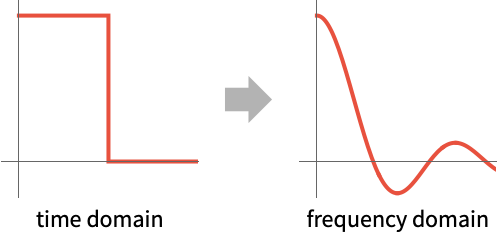
- The Fourier cosine transform is a particular way of viewing the Fourier transform without the need for complex numbers or negative frequencies.
- Joseph Fourier designed his famous transform using this and the Fourier sine transform, and they are still used in applications like signal processing, statistics and image and video compression.
- The Fourier cosine transform of the time domain function
 is the frequency domain function
  for
for  :
: - The Fourier cosine transform of a function
 is by default defined to be
  .
. - The multidimensional Fourier cosine transform of a function
 is by default defined to be
  or when using vector notation,
 ![(2/pi)^(n/2)int_(t in TemplateBox[{}, PositiveReals]^n) f(t) cos(omega t)dt](Files/FourierCosTransform.en/11.png "(2/pi)^(n/2)int_(t in TemplateBox[{}, PositiveReals]^n) f(t) cos(omega t)dt") .
. - Different choices of definitions can be specified using the option FourierParameters.
- The integral is computed using numerical methods if the third argument,
 , is given a numerical value.
 - The asymptotic Fourier cosine transform can be computed using Asymptotic.
- There are several related Fourier transformations:
-
FourierTransform infinite continuous-time functions (FT) FourierSequenceTransform infinite discrete-time functions (DTFT) FourierCoefficient finite continuous-time functions (FS) Fourier finite discrete-time functions (DFT) - The Fourier cosine transform is an automorphism in the Schwartz vector space of functions whose derivatives are rapidly decreasing and thus induces an automorphism in its dual: the space of tempered distributions. These include absolutely integrable functions, well-behaved functions of polynomial growth and compactly supported distributions.
- Hence, FourierCosTransform not only works with absolutely integrable functions on
 , but it can also handle a variety of tempered distributions such as DiracDelta to enlarge the pool of functions or generalized functions it can effectively transform.
 - The lower limit of the integral is effectively taken to be
![TemplateBox[{0, -}, Superscript]](Files/FourierCosTransform.en/14.png "TemplateBox[{0, -}, Superscript]") , so that the Fourier cosine transform of the Dirac delta function
, so that the Fourier cosine transform of the Dirac delta function  is equal to
  . »
. » - The following options can be given:
-
AccuracyGoal Automatic digits of absolute accuracy sought Assumptions $Assumptions assumptions to make about parameters FourierParameters {0,1} parameters to define the Fourier cosine transform GenerateConditions False whether to generate answers that involve conditions on parameters PerformanceGoal $PerformanceGoal aspects of performance to optimize PrecisionGoal Automatic digits of precision sought WorkingPrecision Automatic the precision used in internal computations - Common settings for FourierParameters include:
-
{0,1} 
{1,1} 
{-1,1} 
{0,2Pi} 
{a,b} 
Examples
open all close allBasic Examples (6)
Compute the Fourier cosine transform of a function:
FourierCosTransform[UnitBox[t - 1 / 2], t, ω]Plot the function and its Fourier cosine transform:
{Plot[UnitBox[t - 1 / 2], {t, 0, 2}, Exclusions -> None], Plot[%, {ω, 0, 10}]}Fourier cosine transform of reciprocal square root:
FourierCosTransform[1 / Sqrt[t], t, ω]For a different convention, change the parameters:
FourierCosTransform[1 / Sqrt[t], t, ω, FourierParameters -> {1, 2π}]Fourier cosine transform of a Gaussian is another Gaussian:
FourierCosTransform[E ^ (-t ^ 2), t, ω]{Plot[E ^ (-t ^ 2), {t, 0, 5}, PlotRange -> Full], Plot[%, {ω, 0, 5}, PlotRange -> Full]}Compute the Fourier cosine transform of a multivariate function:
FourierCosTransform[1 / Sqrt[x ^ 2 + y ^ 2], {x, y}, {u, v}]Plot3D[%, {u, 0, 2}, {v, 0, 2}, PlotRange -> {0, 10}, Mesh -> None]Compute the transform at a single point:
FourierCosTransform[Exp[-t ^ 2] Sin[t], t, 0.3]Scope (39)
Basic Uses (3)
Fourier cosine transform of a function for a symbolic parameter ![]() :
:
FourierCosTransform[HeavisideTheta[t], t, ω]Fourier cosine transforms involving trigonometric functions:
FourierCosTransform[Sin[t] / (t E ^ t), t, ω]Plot[%, {ω, 0, 4}]FourierCosTransform[Cos[α t ^ 2], t, ω, Assumptions -> α > 0]Plot[% /. α -> 1 / 4, {ω, 0, 4}]Evaluate the Fourier cosine transform for a numerical value of the parameter ![]() :
:
FourierCosTransform[Exp[-t] / Sqrt[t], t, 1.3]Algebraic Functions (4)
Fourier cosine transform of power functions:
FourierCosTransform[t ^ (n - 1), t, ω, Assumptions -> 0 < n < 1]Cosine transform for rational functions:
FourierCosTransform[1 / (1 + t ^ 2), t, ω]Plot[%, {ω, 0, 4}]FourierCosTransform[t / (1 + t ^ 2), t, ω]Plot[%, {ω, 0, 4}]Fourier cosine transform of a quotient of two nonlinear polynomials:
FourierCosTransform[(1 - t ^ 2) / (t ^ 2 + 1) ^ 2, t, ω]//TrigToExpPlot[%, {ω, 0, 4}]Fourier cosine transform of a quotient of quadratic and quartic polynomials:
FourierCosTransform[t ^ 2 / (t ^ 4 + 1), t, ω]Plot[%, {ω, 0, 10}]Exponential and Logarithmic Functions (3)
Fourier cosine transform of an exponential function:
FourierCosTransform[Exp[-α t], t, ω, Assumptions -> Re[α] > 0]FourierCosTransform[Exp[-3t], t, ω]Plot[%, {ω, 0, 4}]Fourier cosine transforms of products of exponential and trigonometric functions:
FourierCosTransform[Exp[α t] Sin[ β t], t, ω, Assumptions -> {α < 0, β > 0}]Plot[% /. {α -> 3 / 4, β -> 1 / 4}, {ω, 0, 4}]FourierCosTransform[Exp[-t ^ 2] Sin[t], t, ω]Plot[%, {ω, 0, 4}]Cosine transforms of logarithmic functions:
FourierCosTransform[Log[t]UnitBox[t - 1 / 2], t, ω]Plot[%, {ω, 0, 10}]FourierCosTransform[Log[t] / Sqrt[t], t, ω]Plot[%, {ω, 0, 4}]FourierCosTransform[Log[1 + t] / t, t, ω]Plot[%, {ω, 0, 4}]FourierCosTransform[Log[1 + 9 / t ^ 2], t, ω]Plot[%, {ω, 0, 4}]Trigonometric Functions (5)
Expressions involving trigonometric functions:
FourierCosTransform[Sin[2t] ^ 2 / t ^ 2, t, ω]Plot[%, {ω, 0, 4}]Composition of elementary functions:
FourierCosTransform[Cos[α t ^ 2], t, ω, Assumptions -> α > 0]Plot[% /. α -> 3 / 4, {ω, 0, 10}]Ratio of sine and product of exponential and linear functions:
FourierCosTransform[(Sin[t]/t Exp[t]), t, ω]Plot[%, {ω, 0, 10}]Fourier cosine transform of arctangent functions:
FourierCosTransform[ArcTan[2 / t], t, ω]Plot[%, {ω, 0, 10}]FourierCosTransform[ArcTan[2 / t ^ 2], t, ω]Plot[%, {ω, 0, 4}]Fourier cosine transform of Sech is another Sech:
FourierCosTransform[Sech[t], t, ω]Plot[%, {ω, 0, 4}]Special Functions (7)
Sinc function:
FourierCosTransform[Sinc[t], t, ω]Plot[%, {ω, 0, 4}, Exclusions -> None]Fourier cosine transforms of expressions involving ExpIntegralEi:
FourierCosTransform[ExpIntegralEi[-t], t, ω]Plot[%, {ω, 0, 4}]Expression involving Erfc:
FourierCosTransform[t Erfc[α t], t, ω, Assumptions -> α > 0]Plot[% /. α -> 2, {ω, 0, 10}]Expression involving SinIntegral:
FourierCosTransform[SinIntegral[t] - π / 2, t, ω]Plot[%, {ω, 0, 10}]FourierCosTransform[CosIntegral[α t], t, ω, Assumptions -> {α > 0, ω > α}]Plot[%, {ω, 0, 4}]Cosine transforms for BesselJ functions:
FourierCosTransform[BesselJ[0, α t], t, ω, Assumptions -> {α > 0, 0 < ω < α}]Plot[% /. α -> 2, {ω, 0, 2.5}]FourierCosTransform[BesselJ[2 n, α t], t, ω, Assumptions -> {α > 0, 0 < ω < α}]Plot[% /. {α -> 2, n -> 2}, {ω, 0, 2.5}]FourierCosTransform[BesselJ[n, α t] / t ^ n, t, ω, Assumptions -> {α > 0, 0 < ω < α, n∈PositiveIntegers}]Plot[% /. {α -> 2, n -> 2}, {ω, 0, 2.5}]FourierCosTransform[BesselJ[0, Sqrt[t]], t, ω]Plot[%, {ω, 0, 4}]Cosine transforms for BesselY functions:
FourierCosTransform[BesselY[0, α t], t, ω, Assumptions -> {α > 0, ω > α}]Plot[% /. α -> 2, {ω, 0, 4}]FourierCosTransform[BesselY[n, α t] t ^ n, t, ω, Assumptions -> {α > 0, ω > α, Abs[Re[n]] < 1 / 2}]Plot[% /. {α -> 2, n -> 1 / 3}, {ω, 0, 4}]Piecewise Functions and Distributions (4)
Fourier cosine transform of a piecewise function:
f[t_] = Piecewise[{{t, 0 ≤ t ≤ 1}, {0, t > 1}}];
Plot[f[t], {t, 0, 1.5}, Exclusions -> None]FourierCosTransform[f[t], t, ω]Restriction of a sine function to a half-period:
Plot[Sin[α t]UnitBox[α t / π - 1 / 2] /. α -> 3π / 2, {t, 0, 1}]Simplify[FourierCosTransform[Sin[α t]UnitBox[α t / π - 1 / 2], t, ω], α > π]f[t_] = Piecewise[{{t, 0 ≤ t ≤ 1}, {2 - t, 1 < t ≤ 2}, {0, 2 < t }}];
Plot[f[t], {t, 0, 3}]FourierCosTransform[f[t], t, ω]Transforms in terms of FresnelC:
FourierCosTransform[UnitStep[t - 1] / Sqrt[t], t, ω]Plot[%, {ω, 0, 4}]FourierCosTransform[(1 - UnitStep[t - 1]) / Sqrt[t], t, ω]Plot[%, {ω, 0, 4}]Periodic Functions (2)
Fourier cosine transform of cosine:
FourierCosTransform[Cos[t], t, ω]Fourier cosine transform of SquareWave:
Plot[SquareWave[t + 1 / 4], {t, 0, 4}, Exclusions -> None]FourierCosTransform[SquareWave[t + 1 / 4], t, ω]Generalized Functions (4)
Fourier cosine transforms of expressions involving HeavisideTheta:
Plot[HeavisideTheta[t - 1], {t, 0, 2}, Exclusions -> None]FourierCosTransform[HeavisideTheta[t - 1], t, ω]Plot[t HeavisideTheta[t] HeavisideTheta[1 - t], {t, 0, 1.5}, Exclusions -> None]FourierCosTransform[t HeavisideTheta[t] HeavisideTheta[1 - t], t, ω]Fourier cosine transforms involving DiracDelta:
FourierCosTransform[DiracDelta[t], t, ω]Plot[%, {ω, 0, 4}]FourierCosTransform[DiracDelta[t - 1], t, ω]Plot[%, {ω, 0, 4}]FourierCosTransform[DiracDelta'[t - 1], t, ω]Plot[%, {ω, 0, 4}]Fourier cosine transform involving HeavisideLambda:
Plot[HeavisideLambda[t - 1], {t, 0, 4}]FourierCosTransform[HeavisideLambda[t - 1], t, ω]Fourier cosine transform involving HeavisidePi:
Plot[HeavisidePi[t - (3/2)], {t, 0, 3}, Exclusions -> None]FourierCosTransform[HeavisidePi[t - (3/2)], t, ω]Multivariate Functions (2)
Fourier cosine transforms of exponentials in two variables:
FourierCosTransform[Exp[-x - y], {x, y}, {u, v}]{Plot3D[Exp[-x - y], {x, 0, 5}, {y, 0, 5}, Mesh -> None], Plot3D[%, {u, 0, 5}, {v, 0, 5}, Mesh -> None]}FourierCosTransform[Exp[-x ^ 2 - y ^ 2], {x, y}, {u, v}]{Plot3D[Exp[-x ^ 2 - y ^ 2], {x, 0, 5}, {y, 0, 5}, Mesh -> None], Plot3D[%, {u, 0, 5}, {v, 0, 5}, Mesh -> None]}Fourier cosine transform of product of exponential and SquareWave:
Plot3D[E ^ (-x)SquareWave[y + 1 / 4], {x, 0, 5}, {y, 0, 5}, Mesh -> None]FourierCosTransform[E ^ (-x)SquareWave[y + 1 / 4], {x, y}, {u, v}]Formal Properties (3)
Fourier cosine transform of a first-order derivative:
FourierCosTransform[f'[t], t, ω]Fourier cosine transform of a second-order derivative:
FourierCosTransform[f''[t], t, ω]Fourier cosine transform threads itself over equations:
FourierCosTransform[f'[t] == 1 / (t ^ 2 + 1), t, ω]Numerical Evaluation (2)
Calculate the Fourier cosine transform at a single point:
FourierCosTransform[(1/Sqrt[t]), t, .9]Alternatively, calculate the Fourier cosine transform symbolically:
FourierCosTransform[(1/Sqrt[t]), t, ω]Then evaluate it for specific value of ![]() :
:
N[% /. ω -> .9]Options (8)
AccuracyGoal (1)
The option AccuracyGoal sets the number of digits of accuracy:
exact = FourierTransform[HeavisideLambda[t - 1], t, 9 / 10]FourierTransform[HeavisideLambda[t - 1], t, .9, AccuracyGoal -> 5] - exactFourierTransform[HeavisideLambda[t - 1], t, .9] - exactAssumptions (1)
Fourier cosine transform of BesselJ is a piecewise function:
FourierCosTransform[BesselJ[0, t], t, ω, Assumptions -> ω > 1]FourierCosTransform[BesselJ[0, t], t, ω, Assumptions -> ω < 1]FourierParameters (3)
Fourier cosine transform for the unit box function with different parameters:
params = {{0, 1}, {1, 1}, {-1, 1}, {0, 2 π}};
funs = funs = Table[FourierCosTransform[UnitBox[t - (1/2)], t, ω, FourierParameters -> p], {p, params}]
Create a nicely formatted table of the results:
header = { "Parameters", HoldForm@FourierCosTransform[UnitBox[t - (1/2)], t, ω]};
Grid[Prepend[Transpose[{params, funs}], header], IconizedObject[«Grid options»]]//TraditionalForm
Use a nondefault setting for a different definition of transform:
FourierCosTransform[Exp[-t], t, ω, FourierParameters -> {1, 1}]To get the inverse, use the same FourierParameters setting:
InverseFourierCosTransform[%, ω, t, FourierParameters -> {1, 1}]Set up your particular global choice of parameters once per session:
SetOptions[FourierCosTransform, FourierParameters -> {0, 2π}]FourierCosTransform[1, t, ω]//TraditionalFormSetOptions[FourierCosTransform, FourierParameters -> {0, 1}]GenerateConditions (1)
Use GenerateConditionsTrue to get parameter conditions for when a result is valid:
FourierCosTransform[Exp[α t], t, ω, GenerateConditions -> True]PrecisionGoal (1)
The option PrecisionGoal sets the relative tolerance in the integration:
exact = FourierCosTransform[8 / (t ^ 2 + 1), t, 1 / 2]FourierCosTransform[8 / (t ^ 2 + 1), t, .5, PrecisionGoal -> 2] - exactFourierCosTransform[8 / (t ^ 2 + 1), t, .5] - exactWorkingPrecision (1)
If a WorkingPrecision is specified, the computation is done at that working precision:
exact = FourierCosTransform[8 / (t ^ 2 + 1), t, 1 / 2]FourierCosTransform[8 / (t ^ 2 + 1), t, .5, WorkingPrecision -> 18] - exactFourierCosTransform[8 / (t ^ 2 + 1), t, .5] - exactApplications (4)
Ordinary Differential Equations (1)
Consider the following ODE with initial condition ![]() :
:
OdEqn = y''[t] + Ω^2y[t] == Cos[t]Apply the Fourier cosine transform to the ODE:
FourierCosTransform[OdEqn, t, ω]Solve for the Fourier cosine transform of ![]() :
:
SolveValues[%, FourierCosTransform[y[t], t, ω]][[1]] /. y'[0] -> 1Find the inverse Fourier cosine transform with ![]() and
and ![]() :
:
icf[t_] = InverseFourierCosTransform[%, ω, t] /. {κ -> 1, Ω -> 1 / 2}//TrigToExpCompare with DSolveValue:
DSolveValue[{OdEqn /. {κ -> 1, Ω -> 1 / 2}, y'[0] == 1, y[0] == icf[0]}, y[t], t]//TrigToExpPartial Differential Equations (1)
Solve the heat equation for ![]() ,
, ![]() :
: ![]() with initial condition
with initial condition ![]() for
for ![]() and Neumann boundary condition
and Neumann boundary condition ![]() for
for ![]() .
.
eqn = D[u[x, t], t] == α ^ 2 D[u[x, t], x, x];Apply the Fourier cosine transform to the ODE on ![]() :
:
FourierCosTransform[eqn, x, ω]DSolveValue[{D[u1[ω, t], t] == α^2 (-ω^2u1[ω, t] - Sqrt[(2/π)] u^(1, 0)[0, t]), u1[ω, 0] == FourierCosTransform[f[x], x, ω][ω]}, u1[ω, t], t] /. {u^(1, 0)[0, K[1]] -> g[K[1]]}//ExpandCompute the inverse cosine transform of the exponential functions:
h[x_] = InverseFourierCosTransform[Sqrt[(2/π)]E^-t α^2 ω^2, ω, x];
l[x] = InverseFourierCosTransform[-Sqrt[(2/π)]α^2E^(K[1] - t) α^2 ω^2 , ω, x];
The convolution property gives the inverse cosine transform of the first summand to get the solution:
1 / 2Integrate[f[τ](h[x + τ] + h[x - τ]), {τ, 0, ∞}] + Integrate[l[x]g[K[1]], {K[1], 0, t}]Consider the special case with ![]() ,
, ![]() and
and ![]() :
:
% /. {f -> Function[u, UnitBox[u - 1 / 2]], g -> Function[u, 0], α -> 1}Compare with DSolveValue:
DSolveValue[{eqn /. α -> 1, {u[x, 0] == UnitBox[x - 1 / 2], Derivative[1, 0][u][0, t] == 0}}, u[x, t], {x, t}, Assumptions -> {t > 0 && x > 0}]Plot the initial conditions and solutions for different values of ![]() .
.
Plot[{UnitBox[x - 1 / 2], Evaluate@Table[%, {t, {.005, .1, .3, .8}}]}, {x, 0, 4}, PlotLegends -> {UnitBox[x - 1 / 2], .005, .1, .3, .8}, Exclusions -> None]Evaluation of Integrals (2)
Calculate the following definite integral:
Inactive[Integrate][(1/(ω ^ 2 + 9)(ω ^ 2 + 4)), {ω, 0, ∞}]Fourier cosine transform preserves integration of products over ![]() :
:
Inactive[Integrate][FourierCosTransform[(1/(ω ^ 2 + 9)), ω, t]FourierCosTransform[1 / (ω ^ 2 + 4), ω, t], {t, 0, ∞}]Activate[%]Compare with Integrate:
Integrate[(1/(ω ^ 2 + 9)(ω ^ 2 + 4)), {ω, 0, ∞}]Calculate the following definite integral for ![]() :
:
Inactive[Integrate][(1/(α ^ 2 + ω ^ 2) ^ 2), {ω, 0, ∞}]Compute Fourier cosine transform of an exponential function:
FourierCosTransform[E^-α x, x, ω, Assumptions -> α > 0]Inactive[Integrate][Abs[E^-α x] ^ 2, {x, -∞, ∞}] == Inactive[Integrate][Abs[(Sqrt[(2/π)] α/α^2 + ω^2)] ^ 2, {ω, -∞, ∞}]Integrate[E^-2α x, {x, 0, ∞}, Assumptions -> α > 0] == HoldForm[(2α ^ 2/π)]Inactive[Integrate][( 1/(α^2 + ω^2) ^ 2), {ω, 0, ∞}]Solve for the definite integral:
SolveValues[ReleaseHold[%], Inactive[Integrate][( 1/(α^2 + ω^2) ^ 2), {ω, 0, ∞}]][[1]]Compare with Integrate:
Integrate[( 1/(α^2 + ω^2) ^ 2), {ω, 0, ∞}, Assumptions -> α > 0]Properties & Relations (4)
By default, the Fourier cosine transform of ![]() is:
is:
HoldForm[FourierCosTransform[f[t], t, ω] = HoldForm[Sqrt[2 / π]] * Integrate[f[t]Cos[ω t], {t, 0, ∞}]]//TraditionalFormFor ![]() , the definite integral becomes:
, the definite integral becomes:
Sqrt[2 / π]Integrate[Exp[-t ^ 2]Cos[t]Cos[ω t], {t, 0, ∞}]Compare with FourierCosTransform:
FourierCosTransform[Exp[-t ^ 2]Cos[t], t, ω]//TrigToExp//SimplifyUse Asymptotic to compute an asymptotic approximation:
Asymptotic[Inactive[FourierCosTransform][E ^ (-t ^ 3), t, ω], ω -> 0]FourierCosTransform and InverseFourierCosTransform are mutual inverses:
InverseFourierCosTransform[FourierCosTransform[f[t], t, ω], ω, t]FourierCosTransform[InverseFourierCosTransform[G[ω], ω, t], t, ω]FourierCosTransform[1 / (t ^ 2 + 1), t, ω]InverseFourierCosTransform[%, ω, t]Results from FourierCosTransform and FourierTransform agree for even functions:
FourierCosTransform[Sin[t] / t, t, ω]FourierTransform[Sin[t] / t, t, ω ]Simplify[% - %%, ω > 0]Possible Issues (1)
The result from an inverse Fourier cosine transform may not have the same form as the original:
FourierCosTransform[UnitStep[1 + t] UnitStep[1 - t], t, ω]InverseFourierCosTransform[%, ω, t]Fourier cosine transform may be given in terms of generalized functions such as DiracDelta:
FourierCosTransform[1, t, ω]Neat Examples (2)
Fourier cosine transform as a Meijer function:
FourierCosTransform[t / (t ^ 3 + 1), t, ω]Create a table of basic Fourier cosine transforms:
flist = {t ^ n, E ^ (-a t), Exp[-t ^ 2], Sinc[t], DiracDelta[t - a], Log[t], UnitStep[t], UnitBox[t], t Erfc[a t], ConditionalExpression[BesselJ[2, t], 0 < ω < 1], ConditionalExpression[BesselY[0, a t], ω > a]};Grid[Prepend[{#, Assuming[{a > 0}, Simplify[FourierCosTransform[#1, t, ω]]]}& /@ flist, {f[t], FourierCosTransform[f[t], t, ω]}], IconizedObject[«Grid options»]]//TraditionalFormText
Wolfram Research (1999), FourierCosTransform, Wolfram Language function, https://reference.wolfram.com/language/ref/FourierCosTransform.html (updated 2025).
CMS
Wolfram Language. 1999. "FourierCosTransform." Wolfram Language & System Documentation Center. Wolfram Research. Last Modified 2025. https://reference.wolfram.com/language/ref/FourierCosTransform.html.
APA
Wolfram Language. (1999). FourierCosTransform. Wolfram Language & System Documentation Center. Retrieved from https://reference.wolfram.com/language/ref/FourierCosTransform.html