


ListDensityPlot3D
ListDensityPlot3D[farr]
generates a smooth density plot from an array of values farr.
ListDensityPlot3D[{{x1,y1,z1,f1},…,{xn,yn,zn,fn}}]
generates a density plot with values fi at the specified points {xi,yi,zi}.
Details and Options
- ListDensityPlot3D is also known as volume map.
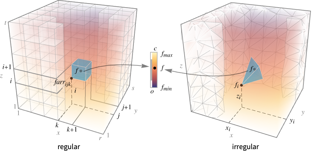
- ListDensityPlot3D works by interpolating the given data into a function
 , then maps the value to a color
  and an opacity
  independently.
 - The opacity function
 is typically used to make some range of values visible, while making some others invisible.
 - For regular data, the function
 has value farr[[i,j,k]] at
  .
. - For irregular data,
 has value fi at
  .
. - The plot visualizes the set
 where
where  is a color function,
  is an opacity function and the region reg is the Cartesian product
  for regular data and the convex hull of {{x1,y1,z1},…,{xn,yn,zn}} for irregular data.
 - farr should be an array of real numbers; positions where farr is not a real number are rendered transparently.
- ListDensityPlot3D[Tabular[…]cspec] extracts and plots values from the tabular object using the column specification cspec.
- The following forms of column specifications cspec are allowed for plotting tabular data:
-
{colx,coly,colz,colf} plot column f against columns x, y and z - ListDensityPlot3D linearly interpolates values so as to give color changes.
- ListDensityPlot3D is mainly intended for continuous values; ArrayPlot3D is intended for purely discrete values.
- ListDensityPlot3D has the same options as Graphics3D, with the following additions and changes: [List of all options]
-
Axes True whether to draw axes BoxRatios {1,1,1} bounding 3D box ratios ColorFunction Automatic how to color the plot ColorFunctionScaling True whether to scale the arguments to ColorFunction DataRange Automatic the range for x, y, and z values to assume MaxPlotPoints Automatic the maximum number of points to include OpacityFunction Automatic how to compute the opacity at each point OpacityFunctionScaling True whether to scale the arguments to OpacityFunction PerformanceGoal $PerformanceGoal aspects of performance to optimize PlotLegends None legends for color gradients PlotRange {Full,Full,Full,Automatic} range of f or other values to include PlotTheme $PlotTheme overall theme for the plot RegionFunction (True&) how to determine whether a point should be included ScalingFunctions None how to scale individual coordinates TargetUnits Automatic desired units to use - ColorFunction and OpacityFunction are supplied with a single argument, given by default by the scaled value of f.
- Typical settings for OpacityFunction include:
-
Automatic automatically determined None no opacity function, fully opaque α constant opacity Opacity[α] Interval[…] make values in the interval more opaque "Image3D" default opacity function used in Image3D func general opacity function - The arguments supplied to RegionFunction are x, y, z, and f.
- The setting DataRange->{{xmin,xmax},{ymin,ymax},{zmin,zmax}} specifies the ranges for x, y, and z coordinates to assume when given an array of f values only as input.
- For an farr of dimension {r,s,t}, the setting DataRangeAutomatic is equivalent to DataRange{{1,r},{1,s},{1,t}}.
- Possible settings for ScalingFunctions include:
-
{sx,sy,sz} scale x, y and z axes - Common built-in scaling functions s include:
-
"Log" 
log scale with automatic tick labeling "Log10" 
base-10 log scale with powers of 10 for ticks "SignedLog" 
log-like scale that includes 0 and negative numbers "Reverse" 
reverse the coordinate direction
List of all options
Examples
open all close allBasic Examples (2)
Plot the density for an array of values:
data = Table[x y z, {z, -1, 1, 2 / 40.}, {y, -1, 1, 2 / 40.}, {x, -1, 1, 2 / 40.}];ListDensityPlot3D[data]Use a different color scheme and legend:
data = Table[Sin[x]Cos[y]Sin[z], {z, -5, 5, 0.1}, {y, -5, 5, 0.1}, {x, -5, 5, 0.1}];ListDensityPlot3D[data, ColorFunction -> "TemperatureMap", PlotLegends -> Automatic]Scope (16)
Data (7)
For regular data consisting of ![]() values, the
values, the ![]() ,
, ![]() , and
, and ![]() data reflects its positions in the array:
data reflects its positions in the array:
data = Table[Sin[x]Cos[y]Sin[z], {z, 0, 2 Pi, 2Pi / 30}, {y, 0, 2Pi, 2Pi / 30}, {x, 0, 2Pi, 2Pi / 30}];ListDensityPlot3D[data]Provide explicit ![]() ,
, ![]() , and
, and ![]() data ranges by using DataRange:
data ranges by using DataRange:
ListDensityPlot3D[data, DataRange -> {{0, 2Pi}, {0, 2Pi}, {0, 2Pi}}]Give explicit ![]() ,
, ![]() ,
, ![]() ,
, ![]() coordinates for points in a density:
coordinates for points in a density:
data = Flatten[Table[{x, y, z, ChessboardDistance[{x, y, z}, {0, 0, 0}]}, {z, -1, 1, 2 / 9}, {y, -1, 1, 2 / 9}, {x, -1, 1, 2 / 9}], 2];ListDensityPlot3D[data]For irregular data ![]() , the
, the ![]() ,
, ![]() , and
, and ![]() data ranges are inferred from data:
data ranges are inferred from data:
pts = RandomPoint[Cuboid[], 10 ^ 3];
data = Table[Append[p, Sqrt[p[[1]] ^ 2 + p[[2]] ^ 2 + p[[3]] ^ 2]], {p, pts}];ListDensityPlot3D[data]Use RegionFunction to constrain data inclusion more generally:
data = Table[x y z, {z, -1, 1, 2 / 40.}, {y, -1, 1, 2 / 40.}, {x, -1, 1, 2 / 40.}];ListDensityPlot3D[data, RegionFunction -> Function[{x, y, z}, x ^ 2 + y ^ 2 + z ^ 2 ≤ 1], DataRange -> {{-1, 1}, {-1, 1}, {-1, 1}}]Plot the density for an array of values given by SparseArray:
data = SparseArray[Flatten[Table[{i ^ 2, j ^ 2, k ^ 2} -> i j k, {i, 1, 4}, {j, 1, 4}, {k, 1, 4}]]];ListDensityPlot3D[data]Plot the density for an array of values given by QuantityArray:
data = QuantityArray[Table[x y z, {z, -1, 1, .05}, {y, -1, 1, .05}, {x, -1, 1, .05}], "kg/m^3"];ListDensityPlot3D[data, AxesLabel -> Automatic, PlotLegends -> Automatic, TargetUnits -> {"Feet", "Feet", "Feet", "g/ft^3"}]Use ClipPlanes to specify one or several clipping planes. In this case, clip ![]() :
:
data = Table[Sin[x]Cos[y]Sin[z], {z, 0, 2 Pi, 2Pi / 30}, {y, 0, 2Pi, 2Pi / 30}, {x, 0, 2Pi, 2Pi / 30}];ListDensityPlot3D[data, ClipPlanes -> {{-1, 1, -1, 2}}, OpacityFunction -> None, DataRange -> {{0, 2Pi}, {0, 2Pi}, {0, 2Pi}}]Tabular Data (1)
tabular = Tabular[IconizedObject[«data»], {"f", "x", "y", "z"}]Plot tabular data in which each column represents data in the form {x,y,z,f}:
ListDensityPlot3D[tabular -> {"x", "y", "z", "f"}]Include a legend for the plot:
ListDensityPlot3D[tabular -> {"x", "y", "z", "f"}, PlotLegends -> Automatic]Presentation (8)
Use PlotTheme to immediately get overall styling:
data = Table[x y z, {z, -1, 1, .05}, {y, -1, 1, .05}, {x, -1, 1, .05}];Table[ListDensityPlot3D[data, PlotLabel -> t, PlotTheme -> t], {t, {"Minimal", "Scientific", "Marketing"}}]Use PlotLegends to get a color bar for the different values:
data = Table[x y z, {z, -1, 1, .05}, {y, -1, 1, .05}, {x, -1, 1, .05}];ListDensityPlot3D[data, PlotLegends -> Automatic]Control the display of axes with Axes:
data = Table[x y z, {z, -1, 1, .05}, {y, -1, 1, .05}, {x, -1, 1, .05}];Table[ListDensityPlot3D[data, PlotLabel -> a, Axes -> a], {a, {True, False, {True, False, True}}}]Label axes using AxesLabel and the whole plot using PlotLabel:
data = Table[x y z, {z, -1, 1, .05}, {y, -1, 1, .05}, {x, -1, 1, .05}];ListDensityPlot3D[data, Ticks -> None, AxesLabel -> {x, y, z}, PlotLabel -> x y z]Color the plot by the function values with ColorFunction:
data = Table[x y z, {z, -1, 1, .05}, {y, -1, 1, .05}, {x, -1, 1, .05}];Table[ListDensityPlot3D[data, PlotLabel -> c, ColorFunction -> c], {c, {Hue, "BlueGreenYellow"}}]Use a custom opacity function to specify the opacity for each point volume:
data = Table[Sin[π x]Sin[π (y + z)], {z, -2, 2, 0.1}, {y, -2, 2, 0.1}, {x, -2, 2, 0.1}];ListDensityPlot3D[data, OpacityFunction -> (If[# < 0.7, 1, 0]&)]TargetUnits specifies which units to use in the visualization:
data = QuantityArray[Table[x y z, {z, -1, 1, .05}, {y, -1, 1, .05}, {x, -1, 1, .05}], "kg/m^3"];ListDensityPlot3D[data, AxesLabel -> Automatic, PlotLegends -> Automatic, TargetUnits -> {"Feet", "Feet", "Feet", "g/ft^3"}]Use ScalingFunctions in the x direction:
ListDensityPlot3D[Table[Sin[π x]Sin[π (y + z)], {z, -2, 2, 0.05}, {y, -2, 2, 0.05}, {x, -2, 2, 0.05}], ScalingFunctions -> {"Log", None, None}]Options (38)
BoxRatios (3)
By default, the edges of the bounding box have the same length:
data = Table[Sin[2π x]Sin[2π y]Sin[2π z], {z, -Pi, Pi, 0.1}, {y, -1, 1, 0.1}, {x, -1, 1, 0.1}];ListDensityPlot3D[data]Use BoxRatiosAutomatic to show the natural scale of the 3D coordinate values:
data = Table[Sin[2π x]Sin[2π y]Sin[2π z], {z, -Pi, Pi, 0.1}, {y, -1, 1, 0.1}, {x, -1, 1, 0.1}];ListDensityPlot3D[data, BoxRatios -> Automatic]Specify the ratios between the bounding box lengths:
data = Table[Sin[2π x]Sin[2π y]Sin[2π z], {z, -Pi, Pi, 0.1}, {y, -1, 1, 0.1}, {x, -1, 1, 0.1}];ListDensityPlot3D[data, BoxRatios -> {5, 2, 3}]ClipPlanes (3)
Use ClipPlanes to specify a clipping plane. In this case, clip ![]() :
:
data = Table[Sin[x + y + z] / 10, {z, 0, 10, .5}, {y, 0, 10, .5}, {x, 0, 10, .5}];ListDensityPlot3D[data, DataRange -> {{0, 10}, {0, 10}, {0, 10}}, OpacityFunction -> None, ClipPlanes -> {{1, 1, -1, 0}}]Specify several clip planes, in this case clipping ![]() and
and ![]() :
:
data = Table[Sin[x + y + z] / 10, {z, 0, 10, .5}, {y, 0, 10, .5}, {x, 0, 10, .5}];ListDensityPlot3D[data, OpacityFunction -> None, ClipPlanes -> {{1, 1, -1, 0}, {0, 1, 0, -4}}, DataRange -> {{0, 10}, {0, 10}, {0, 10}}]Compare to the general RegionFunction:
data = Table[Sin[x + y + z] / 10, {z, 0, 10, .5}, {y, 0, 10, .5}, {x, 0, 10, .5}];ListDensityPlot3D[data, OpacityFunction -> None, RegionFunction -> Function[{x, y, z}, x + y - z ≤ 0], DataRange -> {{0, 10}, {0, 10}, {0, 10}}]ColorFunction (2)
Color by scaled f value at x, y, z coordinates:
data = Table[Sin[(i + j + k) / 20], {i, 0, 20}, {j, 0, 20}, {k, 0, 20}];ListDensityPlot3D[data, ColorFunction -> Hue]Use color functions from ColorData:
data = Table[PDF[DirichletDistribution[{1, 2, 3, 4}], {x, y, z}], {z, 0, 1, 0.05}, {y, 0, 1, 0.05}, {x, 0, 1, 0.05}];Table[ListDensityPlot3D[data, ColorFunction -> cf, DataRange -> {{0, 1}, {0, 1}, {0, 1}}], {cf, {"AlpineColors", "Aquamarine", "ArmyColors", "AtlanticColors"}}]ColorFunctionScaling (2)
Parameters to ColorFunction are normally scaled to be between 0 and 1:
ListDensityPlot3D[Table[x + y + z, {z, 0, 3, 0.2}, {y, 0, 3, 0.2}, {x, 0, 3, 0.2}], ColorFunction -> Hue]Use unscaled coordinates by setting ColorFunctionScaling to False:
data = Table[x + y + z, {z, 0, 3, 0.2}, {y, 0, 3, 0.2}, {x, 0, 3, 0.2}];ListDensityPlot3D[data, ColorFunction -> Hue, ColorFunctionScaling -> False]DataRange (2)
By default, the data range is taken to be the dimension of the array:
data = Table[Exp[-(x ^ 2 + y ^ 2 + z ^ 2)], {z, -1, 1, 1 / 10}, {y, -1, 1, 1 / 20}, {x, -1, 1, 1 / 30}];ListDensityPlot3D[data, DataRange -> Automatic]Explicitly specify the data range:
data = Table[Exp[-(x ^ 2 + y ^ 2 + z ^ 2)], {z, -1, 1, 1 / 10}, {y, -1, 1, 1 / 20}, {x, -1, 1, 1 / 30}];ListDensityPlot3D[data, DataRange -> {{-1, 1}, {-1, 1}, {-1, 1}}]MaxPlotPoints (1)
OpacityFunction (5)
OpacityFunction is Automatic by default:
data = Table[x ^ 2 + y ^ 2 + z ^ 2, {z, -2, 2, 0.1}, {y, -2, 2, 0.1}, {x, -2, 2, 0.1}];ListDensityPlot3D[data]Use None to make the whole volume opaque:
data = Table[Sin[π x]Sin[π (y + z)], {z, -2, 2, 0.1}, {y, -2, 2, 0.1}, {x, -2, 2, 0.1}];ListDensityPlot3D[data, OpacityFunction -> None]Use a custom opacity function to specify the opacity for each point volume:
data = Table[Sin[π x]Sin[π (y + z)], {z, -2, 2, 0.1}, {y, -2, 2, 0.1}, {x, -2, 2, 0.1}];ListDensityPlot3D[data, OpacityFunction -> (If[# < 0.4, 1, 0]&)]Make values in the intervals ![]() and
and ![]() more opaque:
more opaque:
data = Table[Sin[π x]Sin[π y] Sin[π z], {z, -1, 1, 0.05}, {y, -1, 1, 0.05}, {x, -1, 1, 0.05}];ListDensityPlot3D[data, OpacityFunction -> Interval[{-1, -0.6}, {0.6, 1}], OpacityFunctionScaling -> False, PlotLegends -> Automatic, DataRange -> {{-1, 1}, {-1, 1}, {-1, 1}}]Use a constant opacity Opacity[0.05]:
data = Table[Sin[π x]Sin[π y] Sin[π z], {z, -1, 1, 0.05}, {y, -1, 1, 0.05}, {x, -1, 1, 0.05}];ListDensityPlot3D[data, OpacityFunction -> 0.05, PlotLegends -> Automatic, DataRange -> {{-1, 1}, {-1, 1}, {-1, 1}}]OpacityFunctionScaling (2)
By default, scaled values are used:
data = Table[x y z, {z, -5, 5}, {y, -5, 5}, {x, -5, 5}];ListDensityPlot3D[data, OpacityFunction -> Function[f, If[f > 0, 1, 0]]]Use unscaled density values by setting OpacityFunctionScaling to False:
data = Table[x y z, {z, -5, 5}, {y, -5, 5}, {x, -5, 5}];ListDensityPlot3D[data, OpacityFunction -> Function[f, If[f > 0, 1, 0]], OpacityFunctionScaling -> False]PerformanceGoal (2)
Generate a higher-quality plot:
data = Table[x y z, {z, -1, 1, .1}, {y, -1, 1, .1}, {x, -1, 1, .1}];Timing[ListDensityPlot3D[data, PerformanceGoal -> "Quality"]]Emphasize performance, possibly at the cost of quality:
data = Table[x y z, {z, -1, 1, .1}, {y, -1, 1, .1}, {x, -1, 1, .1}];Timing[ListDensityPlot3D[data, PerformanceGoal -> "Speed"]]PlotLegends (2)
No legends are used by default:
data = Table[x y z, {x, -1, 1, 2 / 40.}, {y, -1, 1, 2 / 40.}, {z, -1, 1, 2 / 40.}];ListDensityPlot3D[data]Use PlotLegends->Automatic to show a legended plot:
data = Table[x y z, {z, -1, 1, 2 / 40.}, {y, -1, 1, 2 / 40.}, {x, -1, 1, 2 / 40.}];ListDensityPlot3D[data, PlotLegends -> Automatic]PlotRange (3)
By default, the full plot range is shown:
data = Table[Exp[-(x ^ 2 + y ^ 2 + z ^ 2)], {z, -1, 1, 1 / 20}, {y, -1, 1, 1 / 20}, {x, -1, 1, 1 / 20}];ListDensityPlot3D[data, DataRange -> {{-1, 1}, {-1, 1}, {-1, 1}}]Use specific ranges to show more detail:
data = Table[Exp[-(x ^ 2 + y ^ 2 + z ^ 2)], {z, -1, 1, 1 / 20}, {y, -1, 1, 1 / 20}, {x, -1, 1, 1 / 20}];ListDensityPlot3D[data, DataRange -> {{-1, 1}, {-1, 1}, {-1, 1}}, PlotRange -> {{-1, 0}, All, All}, BoxRatios -> Automatic]Show only function values between 0 and 0.2:
data = Table[Exp[-(x ^ 2 + y ^ 2 + z ^ 2)], {z, -1, 1, 0.05}, {y, -1, 1, 0.05}, {x, -1, 1, 0.05}];ListDensityPlot3D[data, PlotRange -> {All, All, All, {0, 0.2}}]ListDensityPlot3D[data, PlotRange -> {0, 0.2}]PlotTheme (3)
Use a theme with detailed grid lines, ticks, and legends:
data = Table[x y z, {z, -1, 1, 2 / 40.}, {y, -1, 1, 2 / 40.}, {x, -1, 1, 2 / 40.}];ListDensityPlot3D[data, PlotTheme -> "Detailed"]data = Table[x y z, {z, -1, 1, 2 / 40.}, {y, -1, 1, 2 / 40.}, {x, -1, 1, 2 / 40.}];ListDensityPlot3D[data, PlotTheme -> "Detailed", FaceGrids -> None]Compare different plot themes:
data = Table[x y z, {z, -1, 1, 2 / 40.}, {y, -1, 1, 2 / 40.}, {x, -1, 1, 2 / 40.}];Table[ListDensityPlot3D[data, PlotLabel -> t, PlotTheme -> t, ImageSize -> 130], {t, {"Scientific", "Monochrome", "Minimal", "Web", "Working", "Classic", "Business", "Marketing", "Detailed"}}]RegionFunction (3)
data = Table[x y z, {z, -1, 1, 2 / 40.}, {y, -1, 1, 2 / 40.}, {x, -1, 1, 2 / 40.}];ListDensityPlot3D[data, RegionFunction -> Function[{x, y, z}, x ^ 2 + y ^ 2 + z ^ 2 ≤ 1], DataRange -> {{-1, 1}, {-1, 1}, {-1, 1}}]data = Table[x ^ 2 + y ^ 2 - z ^ 2, {z, -2, 2, .2}, {y, -2, 2, .2}, {x, -2, 2, .2}];ListDensityPlot3D[data, RegionFunction -> Function[{x, y, z, f}, f < 2], DataRange -> {{-2, 2}, {-2, 2}, {-2, 2}}]Regions do not have to be connected:
data = Table[x ^ 2 + y ^ 2 - z ^ 2, {z, -2, 2, .2}, {y, -2, 2, .2}, {x, -2, 2, .2}];ListDensityPlot3D[data, RegionFunction -> Function[{x, y, z, f}, x < -1 || x > 1], DataRange -> {{-2, 2}, {-2, 2}, {-2, 2}}]ScalingFunctions (4)
By default, plots have linear scales in all directions:
ListDensityPlot3D[Table[Cos[x + y + z] / 10, {z, 0, 10, .25}, {y, 0, 10, .25}, {x, 0, 10, .25}]]Create a plot with a log-scaled ![]() axis:
axis:
ListDensityPlot3D[Table[Cos[x + y + z] / 10, {z, 0, 10, .25}, {y, 0, 10, .25}, {x, 0, 10, .25}], ScalingFunctions -> {"Log", None, None}]Use ScalingFunctions to scale to reverse the coordinate direction in the ![]() direction:
direction:
ListDensityPlot3D[Table[Cos[x + y + z] / 10, {z, 0, 10, .25}, {y, 0, 10, .25}, {x, 0, 10, .25}], ScalingFunctions -> {None, None, "Reverse"}]Use a scale defined by a function and its inverse:
ListDensityPlot3D[Table[Cos[x + y + z] / 10, {z, 0, 10, .25}, {y, 0, 10, .25}, {x, 0, 10, .25}], ScalingFunctions -> {None, None, {-Log[#]&, Exp[-#]&}}]TargetUnits (1)
Specify which units to use in the visualization:
data = QuantityArray[Table[Exp[-(x ^ 2 + y ^ 2 + z ^ 2)], {z, -2, 2, 0.1}, {y, -2, 2, 0.1}, {x, -2, 2, 0.1}], "Feet"];ListDensityPlot3D[data, TargetUnits -> {"Meters", "Meters", "Meters", "Meters"}, PlotLegends -> Automatic, AxesLabel -> Automatic]Applications (13)
Elementary Functions (4)
data = Table[x, {z, -2, 2}, {y, -2, 2}, {x, -2, 2, 0.25}];ListDensityPlot3D[data]{ListDensityPlot3D[Table[y, {z, -2, 2}, {y, -2, 2, 0.25}, {x, -2, 2}]],
ListDensityPlot3D[Table[z, {z, -2, 2, 0.25}, {y, -2, 2}, {x, -2, 2}]]}{ListDensityPlot3D[Table[x + y, {z, -2, 2}, {y, -2, 2, 0.25}, {x, -2, 2, 0.25}]],
ListDensityPlot3D[Table[y + z, {z, -2, 2, 0.25}, {y, -2, 2, 0.25}, {x, -2, 2}]]}{ListDensityPlot3D[Table[x + y + z, {z, -2, 2, 0.25}, {y, -2, 2, 0.25}, {x, -2, 2, 0.25}]],
ListDensityPlot3D[Table[x - y + z, {x, -2, 2, 0.2}, {y, -2, 2, 0.2}, {z, -2, 2, 0.2}]]}{ListDensityPlot3D[Table[x ^ 2 + y ^ 2, {z, -2, 2}, {y, -2, 2, 0.25}, {x, -2, 2, 0.25}]], ListDensityPlot3D[Table[y ^ 2 + z ^ 2, {z, -2, 2, 0.25}, {y, -2, 2, 0.25}, {x, -2, 2}]]}{ListDensityPlot3D[Table[x ^ 2 + y ^ 2 + z ^ 2, {z, -2, 2, 0.2}, {y, -2, 2, 0.2}, {x, -2, 2, 0.2}]], ListDensityPlot3D[Table[x ^ 2 + y ^ 2 + 2z ^ 2, {z, -2, 2, 0.2}, {y, -2, 2, 0.2}, {x, -2, 2, 0.2}]]}Plot ![]() , a product of univariate functions:
, a product of univariate functions:
ListDensityPlot3D[Table[Sin[π x]Sin[π y]Sin[π z], {z, -2, 2, 0.1}, {y, -2, 2, 0.1}, {x, -2, 2, 0.1}]]Plot ![]() and
and ![]() , univariate and bivariate functions:
, univariate and bivariate functions:
{ListDensityPlot3D[Table[Sin[π x]Sin[π (y + z)], {z, -2, 2, 0.1}, {y, -2, 2, 0.1}, {x, -2, 2, 0.1}]], ListDensityPlot3D[Table[Sin[π (x + y)]Sin[π z], {z, -2, 2, 0.1}, {y, -2, 2, 0.1}, {x, -2, 2, 0.1}]]}ListDensityPlot3D[Table[Sin[π (x + y + z)], {z, -2, 2, 0.1}, {y, -2, 2, 0.1}, {x, -2, 2, 0.1}]]f = Exp[-Norm[{x, y, z} - {-1, -1, -1}]^2] + Exp[-Norm[{x, y, z} - {1, 1, 1}]^2];ListDensityPlot3D[Table[f, {z, -2, 2, 0.2}, {y, -2, 2, 0.2}, {x, -2, 2, 0.2}]]Pick the points ![]() randomly in a box:
randomly in a box:
f = Sum[Exp[-2Norm[{x, y, z} - pi]^2], {pi, RandomPoint[Cuboid[{-1, -1, -1}, {1, 1, 1}], 10]}];ListDensityPlot3D[Table[f, {x, -2, 2, 0.2}, {y, -2, 2, 0.2}, {z, -2, 2, 0.2}]]Simulation Data (6)
Plot a probability density function of three variables:
𝒟 = ProductDistribution[{LogNormalDistribution[0, 1], 3}];
f = PDF[𝒟, {x, y, z}]ListDensityPlot3D[Table[f, {z, 0, 3, .1}, {y, 0, 3, .1}, {x, 0, 3, .1}], DataRange -> {{0, 3}, {0, 3}, {0, 3}}]Simulate the distribution and compute the bin counts:
data = Last@HistogramList[RandomVariate[𝒟, 10 ^ 6], {0, 3, 0.1}];ListDensityPlot3D[data]Simulate a random walk and show the path:
walk = Accumulate[RandomInteger[{-1, 1}, {10 ^ 5, 3}]];Graphics3D[Line[walk], BoxRatios -> 1, Axes -> True]Bin the position that the walk hits in space and show the density:
data = Last@HistogramList[walk];ListDensityPlot3D[data, PlotLegends -> Automatic, DataRange -> CoordinateBounds[walk]]Plot the evolution of two-dimensional cellular automata:
data = CellularAutomaton[{2274, {2, 1}, {1, 1, 1}}, {{{{1}}}, 0}, {20, {{10}}}];ListDensityPlot3D[data]Generate a Menger sponge array:
data = Last@SubstitutionSystem[{1 -> 1 - CrossMatrix[{1, 1, 1}], 0 -> ConstantArray[0, {3, 3, 3}]}, {{{1}}}, 3];ListDensityPlot3D[data, OpacityFunction -> (#&), ColorFunction -> GrayLevel]Plot the evolution of a substitution system:
data = Last@SubstitutionSystem[{1 -> ArrayReshape[IntegerDigits[45115427, 2, 27], {3, 3, 3}], 0 -> ConstantArray[0, {3, 3, 3}]}, {{{1}}}, 3];ListDensityPlot3D[data]Simulate a discrete diffusion model of a two-dimensional array of random values by averaging values of a radius-1 neighborhood in the array:
g[d_] := ArrayFilter[Total[#, 2] / 9&, d, 1];ListDensityPlot3D[NestList[g, RandomReal[1, {40, 40}], 40], PlotLegends -> Automatic, AxesLabel -> {None, None, "time"}]Data Patterns (3)
Visualize the phase for a 3D discrete Fourier transform on data:
data = Arg[Fourier[Table[1 / LCM[i, j, k], {i, 64}, {j, 64}, {k, 64}]]];ListDensityPlot3D[data]Bin the position of atoms in a protein and show the density:
positions = ProteinData["RAB21", "AtomPositions"];data = Last@HistogramList[positions];ListDensityPlot3D[data, PlotLegends -> Automatic]Compare with the molecule plot:
ProteinData["RAB21", "MoleculePlot"]Visualize MRI data from a brain:
data = ExampleData[{"TestImage3D", "MRbrain"}, "GrayLevels"];ListDensityPlot3D[data, BoxRatios -> Automatic]To get the same orientation used by Image3D, use the option DataReversed:
data = ImageData[ExampleData[{"TestImage3D", "MRbrain"}, "Image3D"], DataReversed -> True];ListDensityPlot3D[data, BoxRatios -> Automatic]Properties & Relations (6)
Use ListSliceDensityPlot3D for density plots over slice surfaces:
data = Table[x y z, {z, -2, 2, .1}, {y, -2, 2, .1}, {x, -2, 2, .1}];{ListSliceDensityPlot3D[data, "BackPlanes"], ListDensityPlot3D[data]}Use ListDensityPlot for density plots in 2D:
data = Table[x ^ 2 + y ^ 2, {z, -1, 1, .1}, {y, -1, 1, .1}, {x, -1, 1, .1}];{ListDensityPlot[First[data]], ListDensityPlot3D[data, OpacityFunction -> None]}Use DensityPlot3D for functions:
data = Table[x y z, {z, -1, 1, 0.05}, {y, -1, 1, 0.05}, {x, -1, 1, 0.05}];{DensityPlot3D[x y z, {x, -2, 2}, {y, -2, 2}, {z, -2, 2}], ListDensityPlot3D[data]}Use ListSliceContourPlot3D for contours over slice surfaces:
data = Table[x ^ 2 + y ^ 2 + z ^ 2, {z, -2, 2, .1}, {y, -2, 2, .1}, {x, -2, 2, .1}];{ListSliceContourPlot3D[data], ListDensityPlot3D[data]}Use ListContourPlot3D for constant value surfaces:
data = Table[x ^ 2 + y ^ 2 + z ^ 2, {z, -2, 2, .1}, {y, -2, 2, .1}, {x, -2, 2, .1}];{ListContourPlot3D[data], ListDensityPlot3D[data]}Use ArrayPlot3D for discrete data:
data = Table[GCD[x, y, z] - 1, {z, -5, 5}, {y, -5, 5}, {x, -5, 5}];{ArrayPlot3D[data], ListDensityPlot3D[data]}Text
Wolfram Research (2015), ListDensityPlot3D, Wolfram Language function, https://reference.wolfram.com/language/ref/ListDensityPlot3D.html (updated 2025).
CMS
Wolfram Language. 2015. "ListDensityPlot3D." Wolfram Language & System Documentation Center. Wolfram Research. Last Modified 2025. https://reference.wolfram.com/language/ref/ListDensityPlot3D.html.
APA
Wolfram Language. (2015). ListDensityPlot3D. Wolfram Language & System Documentation Center. Retrieved from https://reference.wolfram.com/language/ref/ListDensityPlot3D.html