



StreamDensityPlot
StreamDensityPlot[{{vx,vy},r},{x,xmin,xmax},{y,ymin,ymax}]
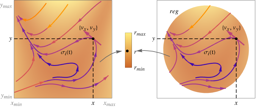
ベクトル場{vx,vy}の流線プロットをスカラー場 r の背景濃度のプロットに重ね合された x と y の関数として生成する.
StreamDensityPlot[{vx,vy},{x,xmin,xmax},{y,ymin,ymax}]
スカラー場がベクトル場のノルムであるとする.
StreamDensityPlot[{{vx,vy},{wx,wy},…,r},{x,xmin,xmax},{y,ymin,ymax}]
複数のベクトル場のプロットを生成する.
StreamDensityPlot[…,{x,y}∈reg]
変数{x,y}が,幾何学領域 reg にあるものと解釈する.
詳細とオプション
- StreamDensityPlotはすべての点におけるベクトル場の局所的方向を示す流線をプロットする.
- StreamDensityPlotは,スカラー場 r の密度プロットを背景とし,そこに重ね合せてベクトル場{vx,vy}の流線プロットを生成する.
- StreamDensityPlotは,
 と
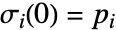 で定義された流線
 をプロットする.
 はベクトルデータの補間関数で,
 は初期流点である.流線
 は点
 を通る曲線で,その接戦は各点におけるベクトル場
 に対応する.
- 流線はスカラー場
 の密度プロットの上に描画される.その初期値はベクトル場
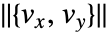 の強度である.
- 流線はベクトル場
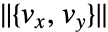 の強度
 に従って彩色される.矢印は
 が大きくなる方向を向く.
- StreamDensityPlotはデフォルトで,プロット全体を通してほぼ一様な密度に達するのに十分な流線を示す.
- StreamDensityPlotは vi等を評価しても実数にならない位置では流線を示さない.
- StreamDensityPlotは,実質的にBlockを使い変数 x と y を局所的なものとして扱う.
- StreamDensityPlotには属性HoldAllがあり,x と y に特定の数値を割り当てた後ではじめて vi等を評価する.
- 場合によっては x と y に特定の数値を割り当てる前にEvaluateを使って vi等を記号的に評価する方がより効率がよいかもしれない.
- StreamDensityPlotにはGraphicsと同じオプションに以下の追加・変更を加えたものが使える. [全オプションのリスト]
- MeshFunctions,RegionFunction,ColorFunction,StreamColorFunction中の関数に渡される引数は x, y, vx, vy, r である.
- デフォルト設定のMeshFunctions->{#5&}では,スカラー場 r にメッシュラインが描かれる.
- 次は,ScalingFunctionsの可能な設定である.
-
{sx,sy} x 軸と y 軸をスケールする - 次は,よく使われる組込みのスケーリング関数 s である.
-
"Log" 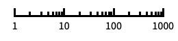
自動目盛ラベル付きの対数スケール "Log10" 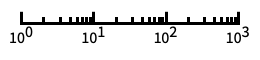
10のベキ乗に目盛が付いた,10を底とする対数スケール "SignedLog" 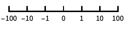
0と負の数を含む対数に似たスケール "Reverse" 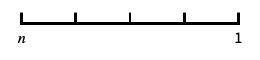
座標の向きを逆にする "Infinite" 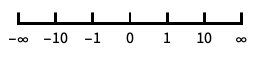
無限スケール
全オプションのリスト
例題
すべて開く すべて閉じる例 (4)
StreamDensityPlot[{-1 - x ^ 2 + y, 1 + x - y ^ 2}, {x, -3, 3}, {y, -3, 3}]StreamDensityPlot[{-1 - x ^ 2 + y, 1 + x - y ^ 2}, {x, -3, 3}, {y, -3, 3}, PlotLegends -> Automatic]場の強度の対数に基づいた背景でベクトル場の流線をプロットする:
StreamDensityPlot[{{-1 - x ^ 2 + y, 1 + x - y ^ 2}, Log[Norm[{-1 - x ^ 2 + y, 1 + x - y ^ 2}] + 1]}, {x, -3, 3}, {y, -3, 3}]最初の場の強度に基づいた背景で2つの場の流線をプロットする:
StreamDensityPlot[{{x, y}, {y, -x}}, {x, -3, 3}, {y, -3, 3}]スコープ (24)
サンプリング (11)

StreamDensityPlot[{{-1 - x ^ 2 + y, 1 + x - y ^ 2}, Cos[x]}, {x, -3, 3}, {y, -3, 3}]2つのベクトル場の流線を,最初のベクトル場の強度に基づいた背景色でプロットする:
StreamDensityPlot[{{x, y}, {y, -x}}, {x, -3, 3}, {y, -3, 3}]Evaluateを使って,数値割当ての前にベクトル場を記号的に評価する:
StreamDensityPlot[Evaluate[D[Sin[x y], {{x, y}}]], {x, 0, 1}, {y, 0, 1}]Table[StreamDensityPlot[{-1 - x ^ 2 + y, 1 + x - y ^ 2}, {x, -3, 3}, {y, -3, 3}, StreamScale -> None, PlotLabel -> p, StreamPoints -> p], {p, {Coarse, Medium, Automatic, Fine}}]StreamDensityPlot[{-1 - x ^ 2 + y, 1 + x - y ^ 2}, {x, -3, 3}, {y, -3, 3}, StreamPoints -> Tuples[{-2, 0, 2}, 2], Epilog -> Point[Tuples[{-2, 0, 2}, 2]]]明示的にシードされた流線のスタイルに自動的なシードと明示的なシードの両方を使う:
StreamDensityPlot[{-1 - x ^ 2 + y, 1 + x - y ^ 2}, {x, -3, 3}, {y, -3, 3}, StreamColorFunction -> None, StreamPoints -> {{{{1, 0}, Red}, {{-1, -1}, Green}, Automatic}}]StreamDensityPlot[{-1 - x ^ 2 + y, 1 + x - y ^ 2}, {x, -3, 3}, {y, -3, 3}, RegionFunction -> Function[{x, y, vx, vy, n}, x y < 0]]StreamDensityPlot[{-1 - x ^ 2 + y, 1 + x - y ^ 2}, {x, -3, 3}, {y, -3, 3}, Mesh -> 5]StreamDensityPlot[{-1 - x ^ 2 + y, 1 + x - y ^ 2}, {x, -3, 3}, {y, -3, 3}, Mesh -> {{2, 4, 5}}]StreamDensityPlot[{{y, -x}, x + y}, {x, y}∈Disk[]]領域はMeshRegionで指定することができる:
𝒟 = MeshRegion[{{0, 0}, {5, -2}, {3, 0}, {5, 2}}, Polygon[{1, 2, 3, 4}]];StreamDensityPlot[{{Sin[x], Cos[y]}, x^2 + y^2}, {x, y}∈𝒟]プレゼンテーション (13)
StreamScaleの設定で異なる破線と鏃を指定する:
Table[StreamDensityPlot[{-1 - x ^ 2 + y, 1 + x - y ^ 2}, {x, -3, 3}, {y, -3, 3}, PlotLabel -> ToString@s, StreamScale -> s], {s, {Automatic, None, 0.2, Full}}]v = {-1 - x ^ 2 + y, 1 + x - y ^ 2};
s = Exp[Norm[v] / 10];Table[StreamDensityPlot[f, {x, -3, 3}, {y, -3, 3}, ColorFunction -> "Pastel"], {f, {v, {v, s}}}]StreamDensityPlot[{-1 - x ^ 2 + y, 1 + x - y ^ 2}, {x, -3, 3}, {y, -3, 3}, StreamColorFunction -> Hue]Table[StreamDensityPlot[{-1 - x ^ 2 + y, 1 + x - y ^ 2}, {x, -3, 3}, {y, -3, 3}, StreamScale -> Full, StreamStyle -> s], {s, {"Toothpick", "Dart", Dashed, Arrowheads[{{0.03, Automatic, Graphics[Circle[]]}}]}}]{StreamDensityPlot[{x, y}, {x, -3, 3}, {y, -3, 3}, PlotTheme -> "Detailed"], StreamDensityPlot[{x, y}, {x, -3, 3}, {y, -3, 3}, PlotTheme -> "Monochrome"]}StreamDensityPlot[{y, -x}, {x, -3, 3}, {y, -3, 3}, StreamMarkers -> "Drop"]StreamDensityPlot[{y, -x}, {x, -3, 3}, {y, -3, 3}, StreamMarkers -> "Drop", StreamStyle -> Blue, StreamColorFunction -> None]StreamDensityPlot[{-1 - x ^ 2 + y, 1 + x - y ^ 2}, {x, -3, 3}, {y, -3, 3}, Mesh -> {{{2, Thick}, {4, Green}, {5, {Thick, Red, Dashed}}}}]Table[StreamDensityPlot[{-1 - x ^ 2 + y, 1 + x - y ^ 2}, {x, -3, 3}, {y, -3, 3}, Mesh -> 10, MeshStyle -> s], {s, {Red, Thick, Directive[Red, Dashed]}}]StreamDensityPlot[{-1 - x ^ 2 + y, 1 + x - y ^ 2}, {x, -3, 3}, {y, -3, 3}, Mesh -> 10, MeshShading -> {Red, Yellow, Green, None}]regionFn = Function[{x, y, vx, vy, n}, 4 < n < 6 || 0 < n < 2];Table[StreamDensityPlot[{-1 - x ^ 2 + y, 1 + x - y ^ 2}, {x, -3, 3}, {y, -3, 3}, RegionFunction -> regionFn, BoundaryStyle -> b], {b, {Red, Thick, Directive[Red, Dashed]}}]StreamDensityPlot[{x, y^2}, {x, -3, 3}, {y, -3, 3}, PlotLegends -> Automatic]StreamDensityPlot[{{x, y}, {y, -x}}, {x, -3, 3}, {y, -3, 3}, StreamColorFunction -> None, PlotLegends -> LineLegend[97, {"one", "two"}]]StreamDensityPlot[{x, y}, {x, 1, 100}, {y, 1, 100}, ScalingFunctions -> {None, "Reverse"}]オプション (85)
Background (1)
BoundaryStyle (2)
ColorFunction (6)
Hueを使って場の強度に彩色する:
StreamDensityPlot[{y, -x}, {x, -3, 3}, {y, -3, 3}, ColorFunction -> Hue] に基づいてHueを使って彩色する:
StreamDensityPlot[{{y, -x}, Sin[x y]}, {x, -3, 3}, {y, -3, 3}, MaxRecursion -> 2, ColorFunction -> Hue]ColorDataから任意の名前付き色階調度を使う:
StreamDensityPlot[{-1 - x ^ 2 + y, 1 + x - y ^ 2}, {x, -3, 3}, {y, -3, 3}, ColorFunction -> "Pastel"]定義済みの色階調度にColorDataを使う:
StreamDensityPlot[{-1 - x ^ 2 + y, 1 + x - y ^ 2}, {x, -3, 3}, {y, -3, 3}, ColorFunction -> Function[{x, y, vx, vy, n}, ColorData["SolarColors"][x y]]]
StreamDensityPlot[{-1 - x ^ 2 + y, 1 + x - y ^ 2}, {x, -3, 3}, {y, -3, 3}, ColorFunction -> Function[{x, y, vx, vy, n}, Blend[{Green, Red}, x]]]ColorFunctionScaling->Falseを使ってスケールされていない値を得る:
StreamDensityPlot[{-1 - x ^ 2 + y, 1 + x - y ^ 2}, {x, -3, 3}, {y, -3, 3}, MaxRecursion -> 4, ColorFunctionScaling -> False, ColorFunction -> Function[{x, y, vx, vy, n}, ColorData[22][Round[n]]]]ColorFunctionScaling (4)
StreamDensityPlot[{y Cos[x y], x Cos[x y]}, {x, -3, 3}, {y, -3, 3}, MaxRecursion -> 2, ColorFunction -> GrayLevel]ColorFunctionScaling->Falseを使ってスケールされていない値を得る:
StreamDensityPlot[{y Cos[x y], x Cos[x y]}, {x, -3, 3}, {y, -3, 3}, MaxRecursion -> 4, ColorFunctionScaling -> False, ColorFunction -> Function[{x, y, vx, vy, n}, ColorData[22][Round[n]]]] 方向にスケールされていない座標を,
 方向にはスケールされた座標を使う:
StreamDensityPlot[{y Cos[x y], x Cos[x y]}, {x, -3, 3}, {y, -3, 3}, ColorFunctionScaling -> {False, True}, ColorFunction -> Function[{x, y, vx, vy, n}, Hue[x, y, 1]]]StreamDensityPlot[{y Cos[x y], x Cos[x y]}, {x, -3, 3}, {y, -3, 3}, MaxRecursion -> 3, ColorFunctionScaling -> {True, True, True, True, False}, ColorFunction -> Function[{x, y, vx, vy, n}, Hue[n, y, 1]]]EvaluationMonitor (2)
ListPlot[Reap[StreamDensityPlot[{-1 - x ^ 2 + y, 1 + x - y ^ 2}, {x, -3, 3}, {y, -3, 3}, EvaluationMonitor :> Sow[{x, y}]]][[-1, 1]]]Block[{k = 0}, StreamDensityPlot[{-1 - x ^ 2 + y, 1 + x - y ^ 2}, {x, -3, 3}, {y, -3, 3}, EvaluationMonitor :> k++];k]MaxRecursion (1)
Mesh (5)
StreamDensityPlot[{-1 - x ^ 2 + y, 1 + x - y ^ 2}, {x, -3, 3}, {y, -3, 3}, Mesh -> None]StreamDensityPlot[{-1 - x ^ 2 + y, 1 + x - y ^ 2}, {x, -3, 3}, {y, -3, 3}, Mesh -> All]StreamDensityPlot[{-1 - x ^ 2 + y, 1 + x - y ^ 2}, {x, -3, 3}, {y, -3, 3}, Mesh -> 5]StreamDensityPlot[{-1 - x ^ 2 + y, 1 + x - y ^ 2}, {x, -3, 3}, {y, -3, 3}, Mesh -> {{2, 4, 5}}]StreamDensityPlot[{-1 - x ^ 2 + y, 1 + x - y ^ 2}, {x, -3, 3}, {y, -3, 3}, Mesh -> {{{2, Thick}, {4, Yellow}, {5, {Thick, Red, Dashed}}}}]MeshFunctions (3)
StreamDensityPlot[{-1 - x ^ 2 + y, 1 + x - y ^ 2}, {x, -3, 3}, {y, -3, 3}, MeshFunctions -> Function[{x, y, vx, vy, n}, n], Mesh -> 5]
StreamDensityPlot[{-1 - x ^ 2 + y, 1 + x - y ^ 2}, {x, -3, 3}, {y, -3, 3}, MeshFunctions -> Function[{x, y, vx, vy, n}, x], Mesh -> 5]StreamDensityPlot[{-1 - x ^ 2 + y, 1 + x - y ^ 2}, {x, -3, 3}, {y, -3, 3}, MeshFunctions -> Function[{x, y, vx, vy, n}, Sqrt[x ^ 2 + y ^ 2]], Mesh -> 5]MeshShading (3)
Noneを使って領域を削除する:
StreamDensityPlot[{-1 - x ^ 2 + y, 1 + x - y ^ 2}, {x, -3, 3}, {y, -3, 3}, Mesh -> 10, MeshShading -> {Red, None}]StreamDensityPlot[{-1 - x ^ 2 + y, 1 + x - y ^ 2}, {x, -3, 3}, {y, -3, 3}, Mesh -> 10, MeshShading -> {Red, Yellow, Green, None}]ColorDataからの指標付きの色を循環的に使う:
StreamDensityPlot[{-1 - x ^ 2 + y, 1 + x - y ^ 2}, {x, -3, 3}, {y, -3, 3}, Mesh -> 10, MeshShading -> ColorData[51, "ColorList"]]MeshStyle (1)
NormalsFunction (2)
StreamDensityPlot[{Cos[x ^ 2 + y], 1 + x - y ^ 2}, {x, -3, 3}, {y, -3, 3}, LightingAngle -> Pi / 4, NormalsFunction -> None]StreamDensityPlot[{Cos[x ^ 2 + y], 1 + x - y ^ 2}, {x, -3, 3}, {y, -3, 3}, LightingAngle -> Pi / 4, NormalsFunction -> Function[{x, y, vx, vy, n}, RandomReal[{0, 1}, {3}]]]PerformanceGoal (2)
PlotLegends (4)
StreamDensityPlot[{y, -x^2}, {x, -3, 3}, {y, -3, 3}]StreamDensityPlot[{y, -x^2}, {x, -3, 3}, {y, -3, 3}, PlotLegends -> Automatic]StreamDensityPlot[{{x, y}, {y, -x}}, {x, -3, 3}, {y, -3, 3}, StreamColorFunction -> None, PlotLegends -> {None, {"one", "two"}}]StreamDensityPlot[{y, -x^2}, {x, -3, 3}, {y, -3, 3}, PlotLegends -> Placed[Automatic, Below]]PlotRange (7)
StreamDensityPlot[{-1 - x ^ 2 + y, 1 + x - y ^ 2}, {x, -3, 3}, {y, -3, 3}, PlotRange -> Full]

StreamDensityPlot[{-1 - x ^ 2 + y, 1 + x - y ^ 2}, {x, -3, 3}, {y, -3, 3}, PlotRange -> 2]
StreamDensityPlot[{-1 - x ^ 2 + y, 1 + x - y ^ 2}, {x, -3, 3}, {y, -3, 3}, PlotRange -> {{-1, 2}, Automatic}]
StreamDensityPlot[{-1 - x ^ 2 + y, 1 + x - y ^ 2}, {x, -3, 3}, {y, -3, 3}, PlotRange -> {{0, Full}, Automatic}]
StreamDensityPlot[{-1 - x ^ 2 + y, 1 + x - y ^ 2}, {x, -3, 3}, {y, -3, 3}, PlotRange -> {Full, {0, 2}}]
StreamDensityPlot[{-1 - x ^ 2 + y, 1 + x - y ^ 2}, {x, -3, 3}, {y, -3, 3}, PlotRange -> {Full, {Full, 5}}]

StreamDensityPlot[{-1 - x ^ 2 + y, 1 + x - y ^ 2}, {x, -3, 3}, {y, -3, 3}, PlotRange -> {{-2, 1.5}, {-1, 2}}]PlotTheme (2)
RegionFunction (3)
StreamDensityPlot[{-1 - x ^ 2 + y, 1 + x - y ^ 2}, {x, -3, 3}, {y, -3, 3}, RegionFunction -> Function[{x, y, vx, vy, n}, x y < 0]]場の強度が指定された閾値を超えている領域のみで流線をプロットする:
StreamDensityPlot[{-1 - x ^ 2 + y, 1 + x - y ^ 2}, {x, -3, 3}, {y, -3, 3}, RegionFunction -> Function[{x, y, vx, vy, n}, n < 6]]StreamDensityPlot[{-1 - x ^ 2 + y, 1 + x - y ^ 2}, {x, -3, 3}, {y, -3, 3}, RegionFunction -> Function[{x, y, vx, vy, n}, 4 < n < 6 || 0 < n < 2]]StreamColorFunction (6)
StreamDensityPlot[{Sin[x], Cos[y]}, {x, -3, 3}, {y, -3, 3}, StreamColorFunction -> Hue]StreamDensityPlot[{{Sin[x], Cos[y]}, x}, {x, -3, 3}, {y, -3, 3}, StreamColorFunction -> Hue]ColorDataから任意の名前付き色階調度を使う:
StreamDensityPlot[{Sin[x], Cos[y]}, {x, -3, 3}, {y, -3, 3}, StreamColorFunction -> "Rainbow"]定義済みの色階調度にColorDataを使う:
StreamDensityPlot[{Sin[x], Cos[y]}, {x, -3, 3}, {y, -3, 3}, StreamColorFunction -> Function[{x, y, vx, vy, n}, ColorData["RedGreenSplit"][x y]]]
StreamDensityPlot[{Sin[x], Cos[y]}, {x, -3, 3}, {y, -3, 3}, StreamColorFunction -> Function[{x, y, vx, vy, n}, Blend[{Green, Red}, x]]]StreamColorFunctionScaling->Falseを使ってスケールされていない値を得る:
StreamDensityPlot[{-1 - x ^ 2 + y, 1 + x - y ^ 2}, {x, -3, 3}, {y, -3, 3}, StreamColorFunctionScaling -> False, StreamColorFunction -> Function[{x, y, vx, vy, n}, ColorData[22][Round[n]]]]StreamColorFunctionScaling (4)
StreamDensityPlot[{Sin[x], Cos[y]}, {x, -3, 3}, {y, -3, 3}, StreamColorFunction -> GrayLevel]StreamColorFunctionScaling->Falseを使ってスケールされていない値を得る:
StreamDensityPlot[{-1 - x ^ 2 + y, 1 + x - y ^ 2}, {x, -3, 3}, {y, -3, 3}, StreamColorFunctionScaling -> False, StreamColorFunction -> Function[{x, y, vx, vy, n}, ColorData[22][Round[n]]]] 方向にスケールされていない座標を,
 方向にはスケールされた座標を使う:
StreamDensityPlot[{Sin[x], Cos[y]}, {x, -3, 3}, {y, -3, 3}, StreamColorFunction -> Function[{x, y, vx, vy, n}, Hue[x, y, 1]], StreamColorFunctionScaling -> {False, True}]StreamDensityPlot[{Sin[x], Cos[y]}, {x, -3, 3}, {y, -3, 3}, StreamColorFunction -> Function[{x, y, vx, vy, n}, Hue[n, y, 1]], StreamColorFunctionScaling -> {True, True, True, True, False}]StreamMarkers (7)
StreamDensityPlot[{y, -x}, {x, -3, 3}, {y, -3, 3}]StreamDensityPlot[{y, -x}, {x, -3, 3}, {y, -3, 3}, StreamMarkers -> "Drop"]StreamDensityPlot[{{y, -x}, {x, y}}, {x, -3, 3}, {y, -3, 3}, StreamMarkers -> {"Drop", "Dart"}]Table[StreamDensityPlot[{-1 - x ^ 2 + y, 1 + x - y ^ 2}, {x, -3, 3}, {y, -3, 3}, PlotLabel -> s, StreamScale -> {Full, All, 0.05}, StreamMarkers -> s], {s, {"Arrow", "ArrowArrow", "CircleArrow"}}]Table[StreamDensityPlot[{-1 - x ^ 2 + y, 1 + x - y ^ 2}, {x, -3, 3}, {y, -3, 3}, PlotLabel -> s, StreamScale -> {Full, All, 0.03}, StreamMarkers -> s], {s, {"BarDot", "Dot", "DotArrow", "DotDot"}}]Table[StreamDensityPlot[{-1 - x ^ 2 + y, 1 + x - y ^ 2}, {x, -3, 3}, {y, -3, 3}, PlotLabel -> s, StreamScale -> {Full, All, 0.03}, StreamMarkers -> s], {s, {"Drop", "BackwardPointer", "Pointer", "Toothpick"}}]Table[StreamDensityPlot[{-1 - x ^ 2 + y, 1 + x - y ^ 2}, {x, -3, 3}, {y, -3, 3}, PlotLabel -> s, StreamScale -> {Full, All, 0.03}, StreamMarkers -> s], {s, {"Dart", "PinDart", "DoubleDart"}}]StreamPoints (6)
StreamDensityPlot[{-1 - x ^ 2 + y, 1 + x - y ^ 2}, {x, -3, 3}, {y, -3, 3}, StreamPoints -> 10]Table[StreamDensityPlot[{-1 - x ^ 2 + y, 1 + x - y ^ 2}, {x, -3, 3}, {y, -3, 3}, StreamPoints -> p, PlotLabel -> p], {p, {Automatic, Coarse, Fine}}]明示的にシードされた流線のスタイルに自動的なシードと明示的なシードの両方を使う:
StreamDensityPlot[{-1 - x ^ 2 + y, 1 + x - y ^ 2}, {x, -3, 3}, {y, -3, 3}, StreamColorFunction -> None, StreamPoints -> {{{{1, 0}, Red}, {{-1, -1}, Green}, Automatic}}]Table[StreamDensityPlot[{-1 - x ^ 2 + y, 1 + x - y ^ 2}, {x, -3, 3}, {y, -3, 3}, PlotLabel -> d, StreamPoints -> {Automatic, d}], {d, {Automatic, 1, Scaled[0.05]}}]Table[StreamDensityPlot[{-1 - x ^ 2 + y, 1 + x - y ^ 2}, {x, -3, 3}, {y, -3, 3}, PlotLabel -> d, StreamPoints -> {Automatic, d}], {d, {Automatic, {Scaled[0.1], Scaled[0.5]}}}]points = Tuples[{-2, 0, 2}, 2]Table[StreamDensityPlot[{-1 - x ^ 2 + y, 1 + x - y ^ 2}, {x, -3, 3}, {y, -3, 3}, StreamPoints -> {points, Automatic, maxlen}, Epilog -> Point[points]], {maxlen, {2.5, Scaled[0.5]}}]StreamScale (9)
StreamDensityPlot[{Sin[x], Cos[y]}, {x, -Pi, Pi}, {y, -Pi, Pi}, StreamPoints -> 10, StreamScale -> Full]StreamDensityPlot[{Sin[x], Cos[y]}, {x, -Pi, Pi}, {y, -Pi, Pi}, StreamPoints -> 10, StreamScale -> None]Table[StreamDensityPlot[{Sin[x], Cos[y]}, {x, -Pi, Pi}, {y, -Pi, Pi}, PlotLabel -> s, StreamScale -> s], {s, {Tiny, Large}}]Table[StreamDensityPlot[{Sin[x], Cos[y]}, {x, -Pi, Pi}, {y, -Pi, Pi}, PlotLabel -> s, StreamScale -> s], {s, {0.1, 0.2, 0.4}}]StreamDensityPlot[{Sin[x], Cos[y]}, {x, -Pi, Pi}, {y, -Pi, Pi}, StreamScale -> {{0.1, 0.1}, Automatic}]Table[StreamDensityPlot[{y, -x}, {x, -Pi, Pi}, {y, -Pi, Pi}, PlotLabel -> n, StreamScale -> {Full, n}], {n, {12, 24, All}}]Table[StreamDensityPlot[{Sin[x], Cos[y]}, {x, -Pi, Pi}, {y, -Pi, Pi}, StreamPoints -> 10, PlotLabel -> a, StreamScale -> {Automatic, Automatic, a}], {a, {.02, .04}}]Table[StreamDensityPlot[{Sin[x], Cos[y]}, {x, -Pi, Pi}, {y, -Pi, Pi}, StreamPoints -> 10, PlotLabel -> a, StreamScale -> {Automatic, Automatic, a}], {a, {Scaled[0.5], Scaled[1], Scaled[1.5]}}]
StreamDensityPlot[{Sin[x], Cos[y]}, {x, -Pi, Pi}, {y, -Pi, Pi}, StreamScale -> {Automatic, 2, Automatic, Function[{x, y, vx, vy, n}, y]}]StreamStyle (5)
StreamStyleでは,StreamColorFunctionは色より優先順位が高い:
StreamDensityPlot[{-1 - x ^ 2 + y, 1 + x - y ^ 2}, {x, -3, 3}, {y, -3, 3}, StreamStyle -> Black]StreamColorFunctionNoneと設定してStreamStyleで色を指定する:
StreamDensityPlot[{-1 - x ^ 2 + y, 1 + x - y ^ 2}, {x, -3, 3}, {y, -3, 3}, StreamStyle -> Black, StreamColorFunction -> None]Table[StreamDensityPlot[{-1 - x ^ 2 + y, 1 + x - y ^ 2}, {x, -3, 3}, {y, -3, 3}, StreamScale -> Full, StreamStyle -> s, StreamColorFunction -> None], {s, {Black, Thick, Directive[Black, Dashed]}}]StreamDensityPlot[{-1 - x ^ 2 + y, 1 + x - y ^ 2}, {x, -3, 3}, {y, -3, 3}, StreamScale -> Full, StreamStyle -> Arrowheads[{{0.03, Automatic, Graphics[Circle[]]}}]]StreamDensityPlot[{{-1 - x ^ 2 + y, 1 + x - y ^ 2}, {-(1 + x - y ^ 2), -1 - x ^ 2 + y}}, {x, -3, 3}, {y, -3, 3}, StreamPoints -> 30, StreamStyle -> {Red, Black}, StreamColorFunction -> None]アプリケーション (16)
f = {Sin[x] ^ 3, -Cos[y] ^ 2};
StreamDensityPlot[Evaluate@{f, Div[f, {x, y}]}, {x, -3, 3}, {y, -3, 3}]f = {Sin[y], -Sin[x] - y / 4};
StreamDensityPlot[Evaluate@{f, Norm[{0, 0, Curl[f, {x, y}]}]}, {x, -3, 3}, {y, -3, 3}]2Dハミルトン(Hamilton)系のハミルトン方程式に重ね合わされた流線を示す:
H[x_, y_] = y ^ 2 / 2 + x ^ 2( x ^ 2 - 2) / 4;
V[x_, y_] = Expand[-Curl[H[x, y], {x, y}]]StreamDensityPlot[{V[x, y], H[x, y]}, {x, -2, 2}, {y, -2, 2}]NDSolveがいかに不変量を保存するかを検証する:
sol = First[NDSolve[{x'[t] == y[t], y'[t] == x[t] - x[t] ^ 3, Thread[{x[0], y[0]} == RandomReal[{-2, 2}, {2}]]}, {x, y}, {t, 0, 10}, InterpolationOrder -> All]];
Plot[Evaluate[(H[x[t], y[t]] - H[x[0], y[0]]) /. sol], {t, 0, 10}]Manipulate[Row[{Text["m"] == MatrixForm[m], StreamDensityPlot[Evaluate[m.{x, y}], {x, -1, 1}, {y, -1, 1}, StreamScale -> Large, StreamColorFunction -> "Rainbow"
]}], {{m, (| | |
| - | - |
| 1 | 0 |
| 0 | 2 |)}, {(| | |
| - | - |
| 1 | 0 |
| 0 | 2 |) -> "Nodal source", (| | |
| - | - |
| 1 | 1 |
| 0 | 1 |) -> "Degenerate source", (| | |
| -- | - |
| 0 | 1 |
| -1 | 1 |) -> "Spiral source", (| | |
| -- | -- |
| -1 | 0 |
| 0 | -2 |) -> "Nodal sink", (| | |
| -- | -- |
| -1 | 1 |
| 0 | -1 |) -> "Degenerate sink", (| | |
| -- | -- |
| 0 | 1 |
| -1 | -1 |) -> "Spiral sink", (| | |
| -- | - |
| 0 | 1 |
| -1 | 0 |) -> "Center", (| | |
| - | -- |
| 1 | 0 |
| 0 | -2 |) -> "Saddle"}}]流線プロットをインタラクティブな微分方程式のデモの背景として使う:
Manipulate[
	splot = StreamDensityPlot[{y, -Sin[x] - .25 y}, {x, -4, 4}, {y, -3, 3}];
	Dynamic[Show[splot,
	ParametricPlot[Evaluate[First[{x[t], y[t]} /. NDSolve[{x'[t] == y[t], y'[t] == -Sin[x[t]] - .25y[t], Thread[{x[0], y[0]} == point]}, {x, y}, {t, 0, T}]]], {t, 0, T}, PlotStyle -> Red]]],
{{T, 10}, 1, 100}, {{point, {1, 0}}, Locator}]fields = | | |
| ---------------------------- | --------------------------------------------------- |
| "positive invariant set" | {y, -x + y(1 - x ^ 2 - 2y ^ 2)} |
| "structurally stable system" | {2x + y - x(x ^ 2 + y ^ 2), -y - y(x ^ 2 + y ^ 2)} |
| "transcritical bifurcation" | {x ^ 2, -y} |
| "reaction-diffusion" | {2(y - x) + x(1 - x ^ 2), -2(y - x) + y(1 - y ^ 2)} |
| "Duffing's equation" | {y, x - x ^ 3} |;fieldIcon[f_] := Image[StreamDensityPlot[f, {x, -3, 3}, {y, -3, 3}, Axes -> False, Frame -> False, ColorFunction -> Hue, StreamPoints -> 20], ImageSize -> 40]TabView[Table[Tooltip[fieldIcon[f[[2]]], f[[1]]] -> StreamDensityPlot[f[[2]], {x, -3, 3}, {y, -3, 3}, StreamScale -> 0.2, ColorFunction -> Hue, PlotLabel -> TraditionalForm[Column@f[[2]]]], {f, fields}]]p[x_, y_] := 169(x - 1) ^ 2 - 16(y - 1) ^ 2 - 153;
q[x_, y_] := 144(x - 1) ^ 2 - 9(y - 1) ^ 2 - 135;With[{λ = 0.8}, StreamDensityPlot[Evaluate@{p[x, y]Cos[λ] - q[x, y]Sin[λ], p[x, y]Sin[λ] + q[x, y]Cos[λ]}, {x, -1, 3}, {y, -1, 3}, StreamScale -> Large, PlotLabel -> Row[{"λ = ", λ}]]]Table[StreamDensityPlot[{2y, 2x - 3x ^ 2 + λ y(x ^ 2 - x ^ 2 + y ^ 2)}, {x, -3, 3}, {y, -3, 3}, PlotLabel -> Row[{"λ = ", λ}]], {λ, {-1, 0, 1, 5}}]f1[x_, y_] := {y, λ1 x + λ2 y + x ^ 3 + x ^ 2 y};Grid@Table[StreamDensityPlot[Evaluate@f1[x, y], {x, -3, 3}, {y, -3, 3}, StreamScale -> Large, StreamStyle -> Black, StreamColorFunction -> None, PlotLabel -> Row[{"λ1 = ", λ1, " λ2 = ", λ2}]], {λ1, {-1, 0, 1}}, {λ2, {-1, 0, 1}}]Manipulateを使ってパラメータ化されたベクトル場を調べる:
Manipulate[StreamDensityPlot[{y, λ + μ x - x ^ 3}, {x, -3, 3}, {y, -3, 3}, StreamScale -> Large, PlotLabel -> {λ, μ}], {λ, -1, 1}, {μ, -1, 1}]Manipulate[StreamDensityPlot[{-x ^ 2 - λ x y ^ 2 + x, -y ^ 3 - λ x ^ 2 y + y}, {x, -3, 3}, {y, -3, 3}, StreamScale -> Large, PlotLabel -> Row[{"λ = ", λ}]], {λ, -5, 5}]Manipulate[StreamDensityPlot[Evaluate[-D[1 / 3(x ^ 3 + y ^ 3) - λ1 x y - λ2 x - λ3 y, {{x, y}}]], {x, -3, 3}, {y, -3, 3}, StreamScale -> Large, PlotLabel -> {λ1, λ2, λ3}], {λ1, -1, 1}, {λ2, -1, 1}, {λ3, -1, 1}]アニメーションのためにラスタライズしたプロットのリストを生成する:
labeledImage[g_, λ_] := Row[{Image[g, ImageSize -> 175], Row[{" λ = ", λ}]}]g = Table[labeledImage[StreamDensityPlot[{y, -1 + λ + Cos[x]}, {x, -3, 3}, {y, -3, 3}, StreamScale -> Large], λ], {λ, -5, 5, 5 / 16}];もとのベクトルグラフィックスの代りにラスタのリストをアニメーションにした方が,メモリが少なくて済むかもしれない:
ListAnimate[g]流線の色をベクトルのノルムの方向にシフトするアニメーションを作成する:
frames = Table[Image[StreamDensityPlot[{-1 - x ^ 2 + y, 1 + x - y ^ 2}, {x, -3, 3}, {y, -3, 3}, StreamScale -> 0.03, StreamColorFunction -> (Hue[k + #5]&)], ImageSize -> 175], {k, 0, 1, 0.1}];ListAnimate[frames]いくつかの例題でさまざまな流線のスタイルとスケールを調べてみる:
fields = {{x + y ^ 2 + y ^ 3, -x + y + y x ^ 2}, {x - x y ^ 2 + y ^ 3, 3y - y x ^ 2 + x ^ 3}, {(2 - x - 2y)x, (2 - 2x - y)y}, {y, (1 - x ^ 2 - y ^ 2)y / 20 - x}, {2 x y, 1 + x ^ 2 - y ^ 2}, {y, x - x ^ 2 + (1 + x)y}};styles = {"Arrow", "ArrowArrow", "CircleArrow", "BarDot", "Dot", "DotDot", "DotArrow", "Dart", "Drop", "BackwardPointer", "Pointer", "Toothpick", "Dart", "PinDart", "DoubleDart", "Segment", "Line"};icons = Table[f -> Image[StreamPlot[f, {x, -3, 3}, {y, -3, 3}, Axes -> False, Frame -> False, StreamPoints -> 20, StreamStyle -> "Line"], ImageSize -> 42], {f, fields}];Manipulate[StreamDensityPlot[field, {x, -3, 3}, {y, -3, 3}, StreamStyle -> style, StreamScale -> scale, ColorFunction -> color, ImageSize -> 300], {style, styles}, {{color, "SandyTerrain"}, ColorData["Gradients"]}, {{scale, 0.2}, 0.05, 0.5, 0.05}, {{field, icons[[1, 1]]}, icons, Setter}]
values = {-1, 0, 1};
plots = MapIndexed[Function[{λ, i}, StreamDensityPlot[{y, -1 + λ + Cos[x]}, {x, -3, 3}, {y, -3, 3}, StreamPoints -> 16, StreamScale -> 0.07, StreamStyle -> ColorData["DeepSeaColors"][0.3i[[1]]]]], values]make3D[GraphicsComplex[pts_, rr___], h_] := GraphicsComplex[PadRight[pts, {Length@pts, 3}, h], rr]make3D[Arrow[pts_, rr___], h_] := Arrow[PadRight[pts, {Length@pts, 3}, h], rr]stackPlots[plots2D : {__Graphics}, dh_, o : OptionsPattern[Graphics3D]] := Graphics3D[MapIndexed[Function[{g, index}, g[[1]] /. p : _GraphicsComplex | _Arrow :> make3D[p, dh index[[1]]]], plots2D], o]plotSpacing = 5;
stackPlots[plots, plotSpacing, Axes -> True, Boxed -> False, Ticks -> {Automatic, Automatic, MapIndexed[{plotSpacing#2[[1]], Row[{"λ = ", #1}]}&, values]}]特性と関係 (12)
データのプロットにListStreamDensityPlotを使う:
data = Table[{-1 - x ^ 2 + y, 1 + x - y ^ 2}, {x, -3, 3, 0.2}, {y, -3, 3, 0.2}];ListStreamDensityPlot[data]StreamPlotを使ってスカラー場のプロットなしで流線だけをプロットする:
StreamPlot[{-1 - x ^ 2 + y, 1 + x - y ^ 2}, {x, -3, 3}, {y, -3, 3}]VectorDensityPlotを使って流線の代りにベクトルで関数をプロットする:
VectorDensityPlot[{-1 - x ^ 2 + y, 1 + x - y ^ 2}, {x, -3, 3}, {y, -3, 3}]ListVectorDensityPlotを使って流線の代りにベクトルでデータをプロットする:
data = Table[{-1 - x ^ 2 + y, 1 + x - y ^ 2}, {x, -3, 3, 0.2}, {y, -3, 3, 0.2}];ListVectorDensityPlot[data]VectorPlotを使ってスカラー場のプロットなしで流線の代りにベクトルでプロットする:
VectorPlot[{-1 - x ^ 2 + y, 1 + x - y ^ 2}, {x, -3, 3}, {y, -3, 3}]VectorPlot3Dを使って3Dベクトル場を可視化する:
VectorPlot3D[{x, y, z}, {x, -1, 1}, {y, -1, 1}, {z, -1, 1}]SliceVectorPlot3Dを使って曲面上に3Dベクトル場を可視化する:
SliceVectorPlot3D[{-y, x, z}, Sphere[], {x, -1, 1}, {y, -1, 1}, {z, -1, 1}]StreamDensityPlotは必要であればより多くの点をサンプルとして使う:
StreamDensityPlot[{y, -x ^ 2}, {x, -3, 3}, {y, -3, 3}, Mesh -> All]スカラー場はDensityPlotを使ってそれ自身でプロットすることができる:
f = {-1 - x ^ 2 + y, 1 + x - y ^ 2};
s = Exp[Norm[f] / 10];{DensityPlot[s, {x, -3, 3}, {y, -3, 3}, ColorFunction -> "Pastel"],
StreamDensityPlot[{f, s}, {x, -3, 3}, {y, -3, 3}, ColorFunction -> "Pastel"]}LineIntegralConvolutionPlotを使ってベクトル場の線形積分たたみ込みをプロットする:
LineIntegralConvolutionPlot[{-1 - x ^ 2 + y, 1 + x - y ^ 2}, {x, -3, 3}, {y, -3, 3}]ComplexVectorPlot[z + 1 / z, {z, 2}]GeoStreamPlotは地球の地図上に流線をプロットする:
GeoStreamPlot[GeoVector[GeoPosition[{{-54.79801473961214, -111.85053058521567},
    {-65.56940402358214, 162.89657500795147}, {-81.67990688759895, -93.36222177594851},
    {7.785750774919734, 95.44840765141487}, {-6.86571958448036, -40.946398330539864},
    { ... 904, "AngularDegrees"]},
   {0.9366099079317551, Quantity[357.70482317743733, "AngularDegrees"]},
   {0.8256817194791912, Quantity[242.07227508889662, "AngularDegrees"]},
   {0.2661401145642981, Quantity[152.90003252279325, "AngularDegrees"]}}]]
特性と関係 (12)
VectorDensityPlotを使って流線ではなくベクトルでプロットする:
VectorDensityPlot[{-1 - x ^ 2 + y, 1 + x - y ^ 2}, {x, -3, 3}, {y, -3, 3}]StreamPlotまたはVectorPlotをスカラー場の密度プロットなしで関数をプロットするのに使う:
{StreamPlot[{-1 - x ^ 2 + y, 1 + x - y ^ 2}, {x, -3, 3}, {y, -3, 3}],
VectorPlot[{-1 - x ^ 2 + y, 1 + x - y ^ 2}, {x, -3, 3}, {y, -3, 3}]}ListStreamDensityPlotを使ってデータをプロットする:
data = Table[{x^2 - y^2, x + y}, {x, -2, 2, 0.1}, {y, -2, 2, 0.1}];ListStreamDensityPlot[data]ListStreamPlotを密度プロットなしのデータのプロットに使う:
ListStreamPlot[data]ListVectorPlotを使って流線の代りにベクトルをプロットする:
ListVectorPlot[data]ListVectorDensityPlotを使ってベクトルに密度プロットを加える:
ListVectorDensityPlot[data]VectorDisplacementPlotを使って変位ベクトル場に関連付けられた領域の変形を可視化する:
VectorDisplacementPlot[{y, x - x^3}, {x, y}∈Disk[], VectorPoints -> Automatic]ListVectorDisplacementPlotを使って同じ変形をデータに基づいて可視化する:
data = Table[{{x, y} = RandomReal[{-1, 1}, {2}], {y, x - x ^ 3}}, {300}];ListVectorDisplacementPlot[data, Disk[], VectorPoints -> Automatic]VectorDisplacementPlot3Dを使って変位ベクトル場に関連付けられた3D領域の変形を可視化する:
VectorDisplacementPlot3D[{y, x, -z}, {x, 0, 1}, {y, 0, 1}, {z, 0, 1}, VectorPoints -> "Boundary"]ListVectorDisplacementPlot3Dを使って同じ変形をデータに基づいて可視化する:
data = Table[{{x, y, z} = RandomReal[{0, 1}, {3}], {y, x, -z}}, {300}];ListVectorDisplacementPlot3D[data, Cuboid[], VectorPoints -> "Boundary"]VectorPlot3DまたはStreamPlot3Dを使って3Dベクトル場を可視化する:
{VectorPlot3D[{z, -x, y}, {x, -1, 1}, {y, -1, 1}, {z, -1, 1}],
StreamPlot3D[{z, -x, y}, {x, -1, 1}, {y, -1, 1}, {z, -1, 1}]}ListVectorPlot3DまたはListStreamPlot3Dを使って同じ3Dベクトル場をデータに基づいて可視化する:
data = Table[{z, -x, y}, {x, -1, 1, .1}, {y, -1, 1, .1}, {z, -1, 1, .1}];{ListVectorPlot3D[data], ListStreamPlot3D[data]}SliceVectorPlot3Dを使って曲面上に3Dベクトル場データを曲面に沿って可視化する:
SliceVectorPlot3D[{x, y, z}, {x, -1, 1}, {y, -1, 1}, {z, -1, 1}]ListSliceVectorPlot3Dを使って同じ3Dベクトル場データをデータに基づいて可視化する:
ListSliceVectorPlot3D[Table[{x, y, z}, {x, -1, 1, .1}, {y, -1, 1, .1}, {z, -1, 1, .1}]]StreamDensityPlotは必要であればより多くの点をサンプルとして使う:
StreamDensityPlot[{y, -x^2}, {x, -3, 3}, {y, -3, 3}, Mesh -> All]スカラー場はListDensityPlotを使ってそれ自身でプロットすることができる:
f = {-1 - x ^ 2 + y, 1 + x - y ^ 2};
s = Exp[Norm[f] / 10];data = Table[{f, s}, {x, -3, 3, 0.2}, {y, -3, 3, 0.2}];
scalarData = Table[s, {x, -3, 3, 0.2}, {y, -3, 3, 0.2}];{ListDensityPlot[scalarData, ColorFunction -> "Pastel"],
ListStreamDensityPlot[data, ColorFunction -> "Pastel"]}ListLineIntegralConvolutionPlotを使ってベクトル場データの線積分のたたみ込みをプロットする:
data = Table[{-1 - x ^ 2 + y, 1 + x - y ^ 2}, {x, -3, 3, .2}, {y, -3, 3, .2}];ListLineIntegralConvolutionPlot[data]ComplexVectorPlotまたはComplexStreamPlotを使って複素変数の複素関数をベクトル場としてまたは流線でプロットする:
{ComplexVectorPlot[Sin[3z], {z, 2}], ComplexStreamPlot[Sin[3z], {z, 2}]}GeoVectorPlotで地図上にベクトルをプロットする:
GeoVectorPlot[GeoVector[GeoPosition[{{-54.79801473961214, -111.85053058521567},
    {-65.56940402358214, 162.89657500795147}, {-81.67990688759895, -93.36222177594851},
    {7.785750774919734, 95.44840765141487}, {-6.86571958448036, -40.946398330539864},
    { ... 904, "AngularDegrees"]},
   {0.9366099079317551, Quantity[357.70482317743733, "AngularDegrees"]},
   {0.8256817194791912, Quantity[242.07227508889662, "AngularDegrees"]},
{0.2661401145642981, Quantity[152.90003252279325, "AngularDegrees"]}}]]GeoStreamPlotでベクトルの代りに流線をプロットする:
GeoStreamPlot[GeoVector[GeoPosition[{{-54.79801473961214, -111.85053058521567},
    {-65.56940402358214, 162.89657500795147}, {-81.67990688759895, -93.36222177594851},
    {7.785750774919734, 95.44840765141487}, {-6.86571958448036, -40.946398330539864},
    { ... 904, "AngularDegrees"]},
   {0.9366099079317551, Quantity[357.70482317743733, "AngularDegrees"]},
   {0.8256817194791912, Quantity[242.07227508889662, "AngularDegrees"]},
   {0.2661401145642981, Quantity[152.90003252279325, "AngularDegrees"]}}]]
おもしろい例題 (3)
vf = {Cos[x + y ^ 3], Sin[y + x ^ 3]};
StreamDensityPlot[Evaluate[{vf, Div[vf, {x, y}]}], {x, -3, 3}, {y, -3, 3}, StreamPoints -> Fine, StreamScale -> Large, ColorFunction -> "Rainbow", MaxRecursion -> 2, StreamStyle -> Black, StreamColorFunction -> None]vf = { 1, Sin[x^3 + y^3]};StreamDensityPlot[Evaluate[{vf, Div[vf, {x, y}]}], {x, -3, 3}, {y, -3, 3}, StreamPoints -> Fine, StreamScale -> Large, ColorFunction -> "Rainbow", MaxRecursion -> 2, StreamStyle -> Black, StreamColorFunction -> None]vf = {Sin[Cos[3 y] + Sin[3 x]], 3 Cos[Cos[3 y] + 3 x]};StreamDensityPlot[Evaluate[{vf, Div[vf, {x, y}]}], {x, -3, 3}, {y, -3, 3}, StreamScale -> Large, ColorFunction -> "Rainbow", MaxRecursion -> 2, StreamStyle -> Black, StreamColorFunction -> None]vf = {Cos[x + y ^ 3], Sin[y + x ^ 3]};
StreamDensityPlot[Evaluate[{vf, Abs[Curl[vf, {x, y}]]}], {x, -2, 2}, {y, -2, 2}, StreamPoints -> Fine, ColorFunction -> "Rainbow", MaxRecursion -> 2, StreamStyle -> Black, StreamScale -> Large, StreamColorFunction -> None]vf = { 1, Sin[x^3 + y^3]};StreamDensityPlot[Evaluate[{vf, Abs[Curl[vf, {x, y}]]}], {x, -3, 3}, {y, -3, 3}, ColorFunction -> "Rainbow", MaxRecursion -> 3, StreamStyle -> Black, StreamColorFunction -> None, StreamPoints -> Fine]vf = {Sin[Cos[3 y] + Sin[3 x]], 3 Cos[Cos[3 y] + 3 x]};
StreamDensityPlot[Evaluate[{vf, Abs[Curl[vf, {x, y}]]}], {x, -3, 3}, {y, -3, 3}, StreamPoints -> Fine, ColorFunction -> "Rainbow", MaxRecursion -> 2, StreamStyle -> Black, StreamColorFunction -> None, StreamScale -> Large]StreamDensityPlot[{y, -x}, {x, -2, 2}, {y, -2, 2}, RegionFunction -> Function[{x, y}, 0.55 < x ^ 2 + y ^ 2 < 4.2], ColorFunction -> "RedBlueTones", Frame -> False, StreamScale -> Medium, BoundaryStyle -> {Cyan, Thick}]StreamDensityPlot[{Cos[x ^ 2 + y], 1 + x - y ^ 2}, {x, -3, 3}, {y, -3, 3}, ColorFunction -> "BeachColors", StreamColorFunction -> "DeepSeaColors", StreamScale -> {Automatic, Automatic, Scaled[0.8]}, Frame -> False, RegionFunction -> Function[(#1 + 3) ≥ 0.45 #2 ^ 2], BoundaryStyle -> {Blue, Thick}]テキスト
Wolfram Research (2008), StreamDensityPlot, Wolfram言語関数, https://reference.wolfram.com/language/ref/StreamDensityPlot.html (2022年に更新).
CMS
Wolfram Language. 2008. "StreamDensityPlot." Wolfram Language & System Documentation Center. Wolfram Research. Last Modified 2022. https://reference.wolfram.com/language/ref/StreamDensityPlot.html.
APA
Wolfram Language. (2008). StreamDensityPlot. Wolfram Language & System Documentation Center. Retrieved from https://reference.wolfram.com/language/ref/StreamDensityPlot.html