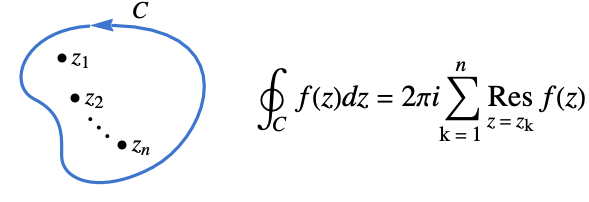
ContourIntegrate[f,z∈cont]
给出 f 沿复平面中由 cont 定义的围道上的积分.
ContourIntegrate
ContourIntegrate[f,z∈cont]
给出 f 沿复平面中由 cont 定义的围道上的积分.
更多信息和选项
- 围道积分也称为路径积分或复线积分.
- 围道积分起源于复分析中对全纯函数和亚纯函数的研究,但现在其应用范围很广,包括拉普拉斯逆变换和 Z 变换的计算、定积分与求和,以及偏微分方程求解等.
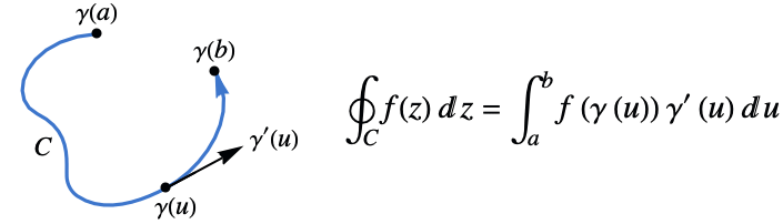
- 函数
沿围道 cont
的围道积分由下式给出: - 围道积分的值与参数化无关,但它确实取决于围道(路径) cont 连续的方向.
- 函数 f 通常是 z 的亚纯函数,但它可以是在复平面中 cont 的邻域中定义的任何分段连续函数.
- 亚纯函数
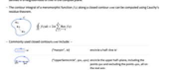
沿闭合路径 cont 的围道积分可以使用柯西留数定理计算. - 常用的闭合路径 cont 包括: »
-
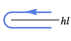
{"Hairpin", hl} 包围半线 hl 

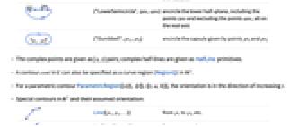
{"UpperSemicircle",ipts,epts} 包围上半平面,包括点 ipts,不包括点 epts,都在实轴上 

{"LowerSemicircle",ipts,epts} 包围下半平面,包括点 ipts,不包括点 epts,都在实轴上 

{"Dumbbell",pt1,pt2} 包围由点 pt1 和 pt2 给出的胶囊 - 复数点以 {x,y} 对的形式给出; 复数半线以 HalfLine 基元的形式给出.
中的围道 cont 也可以指定为
中的曲线区域(RegionQ). - 对于参数围道 ParametricRegion[{x[t],y[t]},{{t,a,b}}],方向是 t 增大的方向.
中的特殊路径及其假定方向:-

Line[{p1,p2,…}] 从 p1 到 p2,等. 
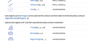
HalfLine[{p1,p1}] 从 p1 朝向 p2 
InfiniteLine[{p1,p2}] 从 p1 朝向 p2 
Circle[p,…] 逆时针 - 可以使用诸如 Polygon 之类的面积区域,这时围道是沿 RegionBoundary[Polygon[…]] 的边界路径.
中的特殊区域及其假设的边界路径方向:-

Triangle[{p1,p2,p3}] 逆时针 
Rectangle[p1,p2] 逆时针 
RegularPolygon[n,…] 逆时针 
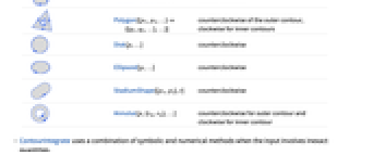
Polygon[{p1,p2,…}{{q1,q2,…},…}] 外围道逆时针,内围道顺时针 
Disk[p,…] 逆时针 
Ellipsoid[p,…] 逆时针 
StadiumShape[{p1,p2},r] 逆时针 
Annulus[p,{rm,rm},…] 外围道逆时针,内围道顺时针 - 当输入涉及不精确的数量时,ContourIntegrate 使用符号和数值方法的组合.
- cont 中的区域可以用 Inactive 封装以防止自动运算.
- 可以给出以下选项:
-
Assumptions $Assumptions 关于参数的假设 GenerateConditions Automatic 是否生成涉及参数条件的答案 PrincipalValue False 是否求柯西主值 WorkingPrecision Automatic 内部计算中使用的精度
范例
打开所有单元 关闭所有单元基本范例 (3)
ContourIntegrate[1 / z, z∈Circle[]]ComplexPlot[(z^3 (1 - 3 z)/(3z + 2) (1 + 2 z^4)), {z, -3 - 3I, 3 + 3I}, ...]ContourIntegrate[(z ^ 3(1 - 3z)/(3z + 2) (1 + 2 z^4)), z∈Circle[{0, 0}, 2]]ContourIntegrate[E ^ (I z) / (z ^ 3 + 1 / 8), z∈RegularPolygon[6]]ComplexPlot[E ^ (I z) / (z ^ 3 + 1 / 8), {z, -2 - 2I, 2 + 2I}, ...]范围 (53)
基本用法 (5)
f = (1/(z - 1)^2 (z - I));ComplexPlot[f, {z, -3 - 3I, 3 + 3I}, ...]ContourIntegrate[f, z∈Circle[{1, 0}, 1]]ContourIntegrate[f, z∈Circle[{1, 0}, 1], WorkingPrecision -> MachinePrecision]f = Exp[2z] / (z - 1);reg = Line[{{0, 0}, {1, 1}, {2, 0}}];ComplexPlot[f, {z, -1 - I, 3 + 3I}, ...]ContourIntegrate[f, z∈reg]f = 1 / (z - a);reg = Disk[{0, 0}, r, {0, Pi}];ContourIntegrate[f, z∈reg]f = Sin[z ^ 2 + 1 / z];reg = Circle[];ContourIntegrate[f, z∈reg, WorkingPrecision -> MachinePrecision]reg = ParametricRegion[{Cos[t], Sin[t]}, {{t, 0, 2Pi}}];ContourIntegrate[1 / z, z∈reg]专题:有理函数 (13)
ContourIntegrate[(3z ^ 3 + 2) / ((z - 1)(z ^ 2 + 9)), z∈Circle[{0, 0}, 4]]ContourIntegrate[z / (z - a) ^ 2, z∈Circle[{0, 0}, 1]]ComplexPlot[(z ^ 5 + 1/(z - I / 2)(z - 1 / 3) ^ 2), {z, -1 - I, 1 + I}, ...]ContourIntegrate[(z ^ 5 + 1/(2z - I)(3z - 1) ^ 3), z∈RegularPolygon[5]]f = (1/(z - 1)(z - 2)(z - 3));reg = Triangle[{{2, 1}, {-2, 0}, {3, -1}}];ComplexPlot[f, {z, -4 - 2I, 4 + 2I}, ...]ContourIntegrate[f, z∈reg]ContourIntegrate[f, z∈reg, WorkingPrecision -> MachinePrecision]f = (z^4 + 1/(z^2 - 1)^2 + 3);reg = Rectangle[{-2, 0}, {2, 1}];ComplexPlot[f, {z, -5 / 2 - 2I, 5 / 2 + 2I}, ...]ContourIntegrate[f, z∈reg]f = 1 / z;reg = Circle[];ComplexPlot[f, {z, -3 / 2 - 3I / 2, 3 / 2 + 3I / 2}, ...]ContourIntegrate[f, z∈reg]f = (1/z^2);reg = Line[{{1, 0}, {2, 1}, {3, 0}, {4, 1}}];ComplexPlot[f, {z, -1 - 2I, 9 / 2 + 2I}, ...]ContourIntegrate[f, z∈reg]f = (1/z - 2);reg = Circle[{0, 0}, {1 / 2, 1}, {0, (7Pi/4)}];ComplexPlot[f, {z, -2 - 2I, 2 + 2I}, ...]ContourIntegrate[f, z∈reg]f = (Cosh[z^2 - 1]/z^3 + I / 2);reg = Disk[{0, 0}, 1, {0, Pi}];ComplexPlot[f, {z, -2 - 2I, 2 + 2I}, ...]ContourIntegrate[f, z∈reg]f = (Cos[1 / z]/z);reg = Circle[];ComplexPlot[f, {z, -2 - 2I, 3 + 2I}, ...]ContourIntegrate[f, z∈reg]f = Exp[1 / Conjugate[z]];reg = Line[{{-1, -1}, {0, -1}, {1, -3 / 2}}];ComplexPlot[f, {z, -2 - 2I, 2 + 2I}, Epilog -> {RGBColor[0.33333333333333337, 0.33333333333333337, 0.33333333333333337], Arrow@reg}, ImageSize -> Small]ContourIntegrate[f, z∈reg]f = Sqrt[z + 1 / 2];reg = Circle[];ComplexPlot[f, {z, -1.5 - 1.5I, 1.5 + 1.5I}, ...]ContourIntegrate[f, z∈reg]f = (z - b) ^ 2 / (z - a);reg = Circle[];ContourIntegrate[f, z∈reg]专题:亚纯函数 (5)
f = (z^2 + I/(z - I / 2)Cos[3z]);reg = RegularPolygon[5];ComplexPlot[f, {z, -2 - 2I, 2 + 2I}, ...]ContourIntegrate[f, z∈reg]N[%]ContourIntegrate[f, z∈reg, WorkingPrecision -> MachinePrecision]f = (Sin[z]/z(z^2 + 3)(z - 2));reg = Circle[{0, 0}, {1, 3}];ComplexPlot[f, {z, -4 - 4I, 4 + 4I}, ...]ContourIntegrate[f, z∈reg]f = (Cosh[z^2 - 1 / 4]/z^2 + 1 / 4);reg = Disk[{0, 0}, 1, {0, Pi}];ComplexPlot[f, {z, -2 - 2I, 2 + 2I}, ...]ContourIntegrate[f, z∈reg]f = Tan[z - I];reg = Annulus[{0, 0}, {1, 3}, {0, Pi}];ComplexPlot[f, {z, -7 / 2 - 7I / 2, 7 / 2 + 7I / 2}, ...]ContourIntegrate[f, z∈reg]ContourIntegrate[1 / Sin[z], z∈Circle[{0, 0}, r], Assumptions -> r > 0]专题:具有本质奇点的函数 (4)
f = Exp[1 / z];reg = Circle[];ComplexPlot[f, {z, -2 - 2I, 2 + 2I}, ...]ContourIntegrate[f, z∈reg]在围道内具有本质奇点的函数 Sin:
f = (Sin[1 / z]/z^4 + I);reg = Rectangle[{-1 / 2, -1 / 2}, {1, 1}];ComplexPlot[f, {z, -2 - 2I, 2 + 2I}, ...]ContourIntegrate[f, z∈reg]f = (Tanh[1 / z]/(z - 1)(z + I / 2));reg = Disk[{-1 / 2, -1}, {1, 3 / 2}, {0, Pi / 2}];ComplexPlot[f, {z, -2 - 2I, 2 + 2I}, ...]ContourIntegrate[f, z∈reg]f = (Cos[2 - 1 / z]/z);reg = Annulus[{-1 / 2, -1}, {1 / 2, 3 / 2}, {0, Pi / 2}];ComplexPlot[f, {z, -2 - 2I, 3 + 2I}, ...]ContourIntegrate[f, z∈reg]专题:非解析函数 (4)
f = Conjugate[z];reg = Circle[];ComplexPlot[f, {z, -2 - 2I, 2 + 2I}, ...]ContourIntegrate[f, z∈reg]Arg 函数的围道积分:
f = Arg[z];reg = Circle[{0, 0}, 2];ComplexPlot[f, {z, -3 - 3I, 3 + 3I}, ...]ContourIntegrate[Arg[z], z∈reg]f = (1/z - Conjugate[z] + 1);reg = Disk[{0, 0}, {1, 2}, {-Pi / 8, 11Pi / 8}];ComplexPlot[f, {z, -2 - 2I, 2 + 2I}, ...]ContourIntegrate[f, z∈reg]//Simplifyf = (Exp[Conjugate[z]]/z + Conjugate[z]);reg = Rectangle[{-5 / 2, -5 / 2}, {-1, -1}];ComplexPlot[f, {z, -6 / 2 - 6 / 2I, 2 + 2I}, ...]ContourIntegrate[f, z∈reg]专题:带分支切割的函数 (2)
f = Sqrt[z];reg = Circle[];ComplexPlot[f, {z, -1.5 - 1.5I, 1.5 + 1.5I}, ...]ContourIntegrate[f, z∈reg]f = (z^2/Sqrt[z^2 + 1 / 2]);reg = Circle[];ComplexPlot[f, {z, -2 - 2I, 2 + 2I}, ...]ContourIntegrate[f, z∈reg]专题:符号参数 (5)
ContourIntegrate[(1/z - a), z∈Circle[{0, 0}, r]]使用 GenerateConditions False 抑制存在条件:
ContourIntegrate[(1/z - a), z∈Circle[{0, 0}, r], GenerateConditions -> False]结果是一个 Piecewise 函数:
ContourIntegrate[(1/(z - a)(z - b)), z∈Circle[{c1, c2}, r]]f = (1/z^2 + a);reg = Disk[{0, 0}, r, {0, Pi}];ContourIntegrate[f, z∈reg, GenerateConditions -> False]ContourIntegrate[(1/z - a), z∈Circle[{c1, c2}, {r1, r2}], GenerateConditions -> False]ContourIntegrate[1 / (z - a), z∈Annulus[{0, 0}, {r, R}, {0, Pi}]]专题:命名围道 (8)
ContourIntegrate[I E ^ (-I p) / (p ^ 2 - 4), p∈{"UpperSemicircle", 2, -2}]ComplexPlot[I E ^ (-I p) / (p ^ 2 - 4), {p, -4 - 4I, 4 + 4I}, ...]ContourIntegrate[I E ^ (-I p x) / (p ^ 2 - e ^ 2) / (p - a), p∈{"UpperSemicircle", Point[{e, 0}], Point[{-e, 0}]}]//SimplifyContourIntegrate[I E ^ (-I p) / (p ^ 2 - 4), p∈{"LowerSemicircle", -2, 2}]ComplexPlot[I E ^ (-I p) / (p ^ 2 - 4), {p, -4 - 4I, 4 + 4I}, ...]ContourIntegrate[I E ^ (-I p x) / (p ^ 2 - e ^ 2) / (p - a), p∈{"LowerSemicircle", Point[{-e, 0}], Point[{e, 0}]}]//SimplifyContourIntegrate[(-z) ^ (1 / 2)E ^ (-z), z∈{"Hairpin", HalfLine[{0, 0}, {1, 0}]}, Assumptions -> Re[z] > 0]ComplexPlot[(-z) ^ (1 / 2)E ^ (-z), {z, -2 - 2I, 3 + 3I}, ...]ContourIntegrate[(-z) ^ (s - 1)E ^ (-z), z∈{"Hairpin", HalfLine[{0, 0}, {1, 0}]}, Assumptions -> Re[s] > 0]ContourIntegrate[(-z) ^ (1 / 3 - 1)E ^ (-z), z∈{"Hairpin", HalfLine[{0, 0}, {1, 0}]}]ComplexPlot[(-z) ^ (1 / 3 - 1)E ^ (-z), {z, -2 - 2I, 3 + 3I}, ...]运算为 Zeta 函数的围道积分:
ContourIntegrate[(-z) ^ (s - 1)E ^ (-a z) / (1 - E ^ -z), z∈{"Hairpin", HalfLine[{0, 0}, {1, 0}]}, Assumptions -> Re[s] > 1]ContourIntegrate[(-z) ^ (14 / 9 - 1)E ^ (-3 z) / (1 - E ^ -z), z∈{"Hairpin", HalfLine[{0, 0}, {1, 0}]}]ComplexPlot[(-z) ^ (14 / 9 - 1)E ^ (-3 z) / (1 - E ^ -z), {z, -3 - 3I, 3 + 3I}, ...]ContourIntegrate[E ^ (-a z) / (1 - E ^ -z), z∈{"Hairpin", HalfLine[{0, 0}, {1, 0}]}]ContourIntegrate[E ^ (-2z) / (1 - E ^ -z), z∈{"Hairpin", HalfLine[{0, 0}, {1, 0}]}]ComplexPlot[E ^ (-2 z) / (1 - E ^ -z), {z, -3 - 3I, 3 + 3I}, ...]ContourIntegrate[E ^ (-z - 1 / 2z ^ 2)(-z) ^ (3 / 2 - 1), z∈{"Hairpin", HalfLine[{0, 0}, {1, 0}]}]ComplexPlot[E ^ (-z - 1 / 2z ^ 2)(-z) ^ (3 / 2 - 1), {z, -3 - 3I, 3 + 3I}, ...]ContourIntegrate[Log[z / (z - 1)], z∈{"Dumbbell", 0, 1}]ComplexPlot[Log[z / (z - 1)], {z, -1 - I, 2 + 2I}, ...]专题:区域围道 (7)
ContourIntegrate[1 / (s + 1)x ^ -s, s∈InfiniteLine[{1, 0}, {0, 1}]]ComplexPlot[1 / (s + 1) * (1 / 2) ^ -s, {s, -20 - 20I, 20 + 20I}, ...]ContourIntegrate[1 / (z - a), z∈Circle[]]ContourIntegrate[1 / (z - 1 / 2), z∈Circle[]]ContourIntegrate[z + 1, z∈Line[{{0, 0}, {1, 1}}]]ComplexPlot[z + 1, {z, -3 - 3I, 3 + 3I}, ...]reg = Triangle[{{0, 1}, {-1, 0}, {1, 0}}];ContourIntegrate[1 / (z - a), z∈reg]//SimplifyContourIntegrate[1 / (z - 1 / 2I), z∈reg]ComplexPlot[1 / (z - 1 / 2I), {z, -2 - I, 2 + 2I}, ...]reg = Rectangle[{-1, -1}, {1, 1}];ContourIntegrate[E ^ (I z) / (z ^ 2 + 1 / 4), z∈reg]ComplexPlot[E ^ (I z) / (z ^ 2 + 1 / 4), {z, -2 - 2I, 2 + 2I}, ...]reg = Disk[{0, 0}, {1, 2}, {0, Pi / 3}];ContourIntegrate[1 / (z - 1 / 2 - I), z∈reg]ComplexPlot[1 / (z - 1 / 2 - I), {z, -1 - I, 2 + 2I}, ...]reg = Annulus[{0, 0}, {1, 2}, {0, Pi}];ContourIntegrate[1 / (z ^ 2 + 3 / 2), z∈reg]ComplexPlot[1 / (z ^ 2 + 3 / 2), {z, -3 - I, 3 + 3I}, ...]选项 (6)
Assumptions (1)
选项 Assumptions 可用于参数:
ContourIntegrate[1 / (z - a), z∈Circle[]]ContourIntegrate[1 / (z - a), z∈Circle[], Assumptions -> Abs[a] < 1]GenerateConditions (2)
ContourIntegrate 使用 GenerateConditionsAutomatic 生成参数条件:
ContourIntegrate[1 / (z - a), z∈Circle[]]使用选项 GenerateConditionsFalse 抑制存在条件:
ContourIntegrate[1 / (z - a), z∈Circle[], GenerateConditions -> False]ContourIntegrate[1 / (z - a), z∈Annulus[{0, 0}, {r, R}]]使用 GenerateConditionsFalse 抑制条件:
ContourIntegrate[1 / (z - a), z∈Annulus[{0, 0}, {r, R}], GenerateConditions -> False]PrincipalValue (1)
选项 PrincipalValue 可用于计算柯西主值:
ContourIntegrate[1 / (z ^ 2 - I), z∈Line[{{0, 0}, {1, 1}}]]ContourIntegrate[1 / (z ^ 2 - I), z∈Line[{{0, 0}, {1, 1}}], PrincipalValue -> True]WorkingPrecision (2)
当设置了 WorkingPrecision 时,积分以数值计算:
f = Exp[Tan[2 + 1 / z]];ContourIntegrate[f, z∈Circle[]]ContourIntegrate[f, z∈Circle[], WorkingPrecision -> MachinePrecision]f = 1 / (z - 0.5);ContourIntegrate[f, z∈Circle[]]应用 (22)
有理函数 (2)
ContourIntegrate[(1/z^2 + 1), z∈Disk[{0, 0}, R, {0, Pi}]]Limit[%, R -> ∞]使用 Integrate 获得相同的结果:
Integrate[(1/x^2 + 1), {x, -∞, ∞}]Integrate[(x^2/(x^2 + 1)(x^2 + 4)), {x, 0, ∞}]ContourIntegrate[(z^2/(z^2 + 1)(z^2 + 4)), z∈Disk[{0, 0}, R, {0, Pi}], Assumptions -> R > 0]Limit[%, R -> ∞]三角有理积 (2)
Integrate[(Cos[2x]/(x^2 + a^2)^2), {x, -∞, ∞}]Integrate[(Sin[2x]/(x^2 + a^2)^2), {x, -∞, ∞}]res = Refine[ContourIntegrate[(Exp[2 I z]/(z^2 + a^2)^2), z∈Disk[{0, 0}, R, {0, Pi}]], Re[a] > 0]Limit[Simplify[Re[res], a > 0], R -> Infinity]Limit[Simplify[Im[res], a > 0], R -> Infinity]Integrate[(x Sin[2x]/x^2 + 3), {x, -∞, ∞}]Integrate[(x Cos[2x]/x^2 + 3), {x, -∞, ∞}]ContourIntegrate[(z Exp[I 2 z]/z^2 + 3), z∈Disk[{0, 0}, R, {0, Pi}]]Limit[%, R -> ∞]{Im[%], Re[%]}三角函数 (3)
f = (1/1 + a Sin[θ]);Integrate[f, {θ, 0, 2Pi}]% /. a -> 1 / 2g = f /. {Sin[θ] -> (z - z^-1/2I)}//FullSimplifyContourIntegrate[(g/I z), z∈Circle[], GenerateConditions -> True]% /. a -> 1 / 2f = (2Cos[2θ]/1 - 2a Cos[θ] + a^2);Integrate[f, {θ, 0, 2Pi}]//Simplifyg = (f//TrigExpand) /. {Sin[θ] -> (z - z^-1/2I), Cos[θ] -> (z + z^-1/2)}//FullSimplifyContourIntegrate[(g/I z), z∈Circle[], GenerateConditions -> True]f = (1/5 + 4Sin[θ]);Integrate[f, {θ, 0, 2Pi}]g = f /. {Sin[θ] -> (z - z^-1/2I)}//FullSimplifyContourIntegrate[(g/I z), z∈Circle[]]傅立叶变换 (2)
FourierTransform[(1/x^2 + 1), x, k](1/Sqrt[2Pi])ContourIntegrate[(Exp[I k z]/z^2 + 1), z∈Disk[{0, 0}, r, {0, Pi}]]Limit[%, r -> Infinity](-1/Sqrt[2Pi])ContourIntegrate[(Exp[I k z]/z^2 + 1), z∈Disk[{0, 0}, r, {-Pi, 0}]]Limit[%, r -> Infinity]FourierTransform[(1/-2 + 2x - x^2), x, k](1/Sqrt[2Pi])ContourIntegrate[(Exp[I k z]/-2 + 2z - z^2), z∈Disk[{0, 0}, r, {0, Pi}]]Limit[%, r -> Infinity](-1/Sqrt[2Pi])ContourIntegrate[(Exp[I k z]/-2 + 2z - z^2), z∈Disk[{0, 0}, r, {-Pi, 0}]]Limit[%, r -> Infinity]拉普拉斯逆变换 (4)
InverseLaplaceTransform[1 / (s + 1), s, t, GenerateConditions -> True]1 / (2Pi I)ContourIntegrate[1 / (s + 1) * E ^ (s t), s∈InfiniteLine[{1, 0}, {0, 1}]]f = Log[(s + 1) / (s + 2)];InverseLaplaceTransform[f, s, t, GenerateConditions -> True]1 / (2Pi I)ContourIntegrate[f * E ^ (s t), s∈InfiniteLine[{1, 0}, {0, 1}]]InverseLaplaceTransform[1 / Sqrt[s + 1], s, t, GenerateConditions -> True]1 / (2Pi I)ContourIntegrate[1 / Sqrt[s + 1] * E ^ (s t), s∈InfiniteLine[{1, 0}, {0, 1}]]包含 Log 的函数的拉普拉斯逆变换:
InverseLaplaceTransform[Log[s] / (s - 1), s, t, GenerateConditions -> True]1 / (2Pi I)ContourIntegrate[Log[s] / (s - 1) * E ^ (s t), s∈InfiniteLine[{1, 0}, {0, 1}]]梅林逆变换 (4)
InverseMellinTransform[(1/s^2 - 1), s, x, GenerateConditions -> True]1 / (2Pi I)ContourIntegrate[x ^ (-s) * (1/s^2 - 1), s∈InfiniteLine[{{2, 0}, {2, 1}}], GenerateConditions -> True]InverseMellinTransform[1 / (s - 1), s, x, GenerateConditions -> True]1 / (2Pi I)ContourIntegrate[1 / (s - 1) * x ^ -s, s∈InfiniteLine[{2, 0}, {0, 1}]]MellinTransform[(1/(1 + x)^3), x, s, GenerateConditions -> True]1 / (2Pi I)ContourIntegrate[Gamma[s]Gamma[3 - s] / 2 * x ^ -s, s∈InfiniteLine[{2, 0}, {0, 1}]]InverseMellinTransform[Gamma[s]Gamma[3 - s] / 2, s, x, GenerateConditions -> True]MellinTransform[(x ^ 2/(1 + x)^3), x, s, GenerateConditions -> True]1 / (2Pi I)ContourIntegrate[(1/2) π s (1 + s) Csc[π s] * x ^ -s, s∈InfiniteLine[{0, 0}, {0, 1}]]InverseMellinTransform[(1/2) π s (1 + s) Csc[π s], s, x]Z 逆变换 (2)
InverseZTransform[z / (z - a), z, n](1/2Pi I)ContourIntegrate[(z^n/(z - a)), z∈Circle[{0, 0}, r]]Refine[%, r > Abs[a]]f = InverseZTransform[z / (z ^ 2 - 3 z + 1), z, n](1/2Pi I)ContourIntegrate[z^n / (z ^ 2 - 3 z + 1), z∈Circle[{0, 0}, r]]//FullSimplifyg = Limit[%, r -> ∞]//FullSimplifyf - g//FullSimplify经典定理 (3)
f = 3z ^ 2 / (z ^ 3 - 1 / 2);reg = Circle[];ComplexPlot[f, {z, -2 - 2I, 2 + 2I}, ...]ContourIntegrate[f, z∈reg](2Pi I) * ResidueSum[{f, Abs[z] < 1}, z]积分围道可以在不改变积分值的情况下变形,前提是函数的奇点不交叉:
f = 1 / (z - 2) + 1 / (z - 3);reg1 = Line[{{-1, 0}, {0, 1}, {1, 0}}];ContourIntegrate[f, z∈reg1]reg2 = Line[{{-1, 0}, {0, -1}, {1, 0}}];ContourIntegrate[f, z∈reg2]ContourIntegrate[1 / (z - 2), z∈Circle[]]ComplexPlot[1 / (z - 2), {z, -3 - 3I, 3 + 3I}, ...]属性和关系 (6)
如果符号计算失败,应用 N[ContourIntegrate[...]] 获得数值解:
f = Exp[Tan[2 + 1 / z]];ContourIntegrate[f, z∈Circle[]]N[%]这也可以使用 NIntegrate 计算:
NIntegrate[I * E ^ (I t) * (f /. z -> E ^ (I t)), {t, 0, 2Pi}]围道积分也可以使用 Integrate 获得:
ContourIntegrate[1 / (z - 1 / 2), z∈Circle[]]Integrate[I * E ^ (I t) / (E ^ (I t) - 1 / 2), {t, 0, 2Pi}]Integrate 可以沿复平面中的直线路径积分:
Integrate[z ^ 2, {z, 0, 1 + I}]ContourIntegrate[z ^ 2, z∈Line[{{0, 0}, {1, 1}}]]闭合路径上的围道积分也可以使用 ResidueSum 获得:
f = z ^ 2 / (2z ^ 3 - 1);ContourIntegrate[f, z∈Circle[{0, 0}, 2]]2πI * ResidueSum[{f, Abs[z] < 2}, z]//Simplify亚纯函数的极点可以使用 FunctionPoles 找到:
f = Cos[z] / (z + a);FunctionPoles[f, z]ContourIntegrate[f, z∈Circle[{0, 0}, 1]]也可以使用 Residue 计算积分:
2π I * Residue[f, {z, -a}]闭合路径上的围道积分也可以使用 Residue 获得:
f = z ^ 2 / ((z - 1)(z - 2));ContourIntegrate[f, z∈Circle[{0, 0}, 3]]2π I * (Residue[f, {z, 1}] + Residue[f, {z, 2}])互动范例 (2)
f = (1/z^2 + 1);Manipulate[
ComplexPlot[f, {z, -6 - 6I, 6 + 6I}, ...]
, {R, 0.1, 7}, SaveDefinitions -> True]Manipulate[ContourIntegrate[f, z∈Disk[{0, 0}, R, {0, Pi}], WorkingPrecision -> MachinePrecision], {R, 0.1, 7}, SaveDefinitions -> True]ContourIntegrate[f, z∈Disk[{0, 0}, R, {0, Pi}]]f = (1/z^6 + 1);Manipulate[
ComplexPlot[f, {z, -6 - 6I, 6 + 6I}, ...], {R, 0.1, 7}, SaveDefinitions -> True]Manipulate[ContourIntegrate[f, z∈Disk[{0, 0}, R, {0, Pi}], WorkingPrecision -> MachinePrecision], {R, 0.1, 7}, SaveDefinitions -> True]ContourIntegrate[f, z∈Disk[{0, 0}, R, {0, Pi}]]巧妙范例 (2)
f = (z + 3 / 2/z^3 - 1 / 2);reg = Disk[{0, 0}, 1, {Pi / 6, 11Pi / 6}];ComplexPlot[f, {z, -2 - 2I, 2 + 2I}, ...]ContourIntegrate[f, z∈reg]reg = Line[{{0, 3}, {1, 1}, {3, 0}, {1, -1}, {0, -3}, {-1, -1}, {-3, 0}, {-1, 1}, {0, 3}}];ComplexPlot[(Exp[z]Cos[z]/(z^5 - 1)(z^3 - 8)), {z, -4 - 4I, 4 + 4I}, ...]ContourIntegrate[(Exp[z]Cos[z]/(z^5 - 1)(z^3 - 8)), z∈reg]相关指南
-
▪
- 复变量函数
文本
Wolfram Research (2023),ContourIntegrate,Wolfram 语言函数,https://reference.wolfram.com/language/ref/ContourIntegrate.html.
CMS
Wolfram 语言. 2023. "ContourIntegrate." Wolfram 语言与系统参考资料中心. Wolfram Research. https://reference.wolfram.com/language/ref/ContourIntegrate.html.
APA
Wolfram 语言. (2023). ContourIntegrate. Wolfram 语言与系统参考资料中心. 追溯自 https://reference.wolfram.com/language/ref/ContourIntegrate.html 年
BibTeX
@misc{reference.wolfram_2026_contourintegrate, author="Wolfram Research", title="{ContourIntegrate}", year="2023", howpublished="\url{https://reference.wolfram.com/language/ref/ContourIntegrate.html}", note=[Accessed: 16-September-2026]}
BibLaTeX
@online{reference.wolfram_2026_contourintegrate, organization={Wolfram Research}, title={ContourIntegrate}, year={2023}, url={https://reference.wolfram.com/language/ref/ContourIntegrate.html}, note=[Accessed: 16-September-2026]}