ComplexArrayPlot[array]
配列 array 中の複素値 zijが,Arg[zij]が色で,Abs[zij]が陰影で示される正方形の離散配列で表示されたプロットを生成する.
ComplexArrayPlot
ComplexArrayPlot[array]
配列 array 中の複素値 zijが,Arg[zij]が色で,Abs[zij]が陰影で示される正方形の離散配列で表示されたプロットを生成する.
詳細とオプション
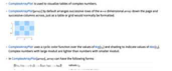
- ComplexArrayPlotは,複素数の表の可視化に使われる.
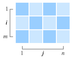
- ComplexArrayPlot[array]は,デフォルトで,ちょうど表や格子が通常フォーマットされるように,mn 次元の array の連続する行をページの下に向かって,連続する列を横に向かって並べる.
- ComplexArrayPlotは,Arg[zij]の値に循環的な色関数を使い,Abs[zij]の値を示すためには陰影を使う.法が大きい複素数は法が小さい数よりも明るい色になる.
- ComplexArrayPlot[array]の array は次の形でよい.
-
{{z11,z12,…,z1n},…,{zm1,zm2,…,zmn}} 値 zij SparseArray 通常の配列としての値 NumericArray 通常の配列としての値 Dataset 通常の配列としての値 - zijには,次の特別な項目を使うことができる.
-
None 背景色 色指示子 指定の色 - array が不調和配列のときは,短い行の右側が背景色で充填されたものとして扱われる.
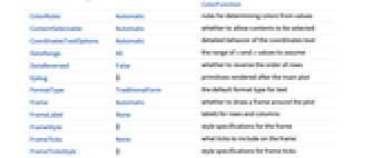
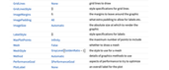
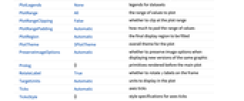
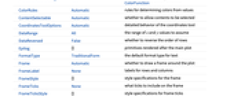
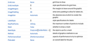
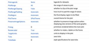
- ComplexArrayPlotには,Graphicsと同じオプションに以下の追加・変更を加えたものが使える. [全オプションのリスト]
-
AspectRatio Automatic 縦横比 ClippingStyle None 値が切り取られたセルをどのように表示するか ColorFunction Automatic 各セルにどのように彩色するか ColorFunctionScaling True ColorFunctionの引数をスケールするかどうか ColorRules Automatic 値から色を決める規則 DataRange All 仮定する
と
の値の範囲DataReversed False 行の順序を逆にするかどうか Frame Automatic プロットの周りに枠を描くかどうか FrameLabel None 行と列のラベル FrameTicks None 枠にどのような目盛を含めるか MaxPlotPoints Infinity 含める点の最大数 Mesh False メッシュを描くかどうか MeshStyle GrayLevel[GoldenRatio-1] メッシュのスタイル PerformanceGoal $PerformanceGoal パフォーマンスのどの面を最適化するか PlotLegends None データ集合の凡例 PlotRange All プロットする値の範囲 PlotTheme $PlotTheme プロットの全体的なテーマ TargetUnits Automatic プロット中に表示する単位 - ColorRulesで与えられる規則は各セルの値
に適用される.規則はパターンを含んでいてもよい. - ColorRulesの中に適用される規則がない場合は,ColorFunctionを使って色が決定される.
- デフォルト設定のColorRules->Automaticでは,ColorRulesの代りに明示的な設定のColorFunctioncfunc が使われる.
- ColorFunction->{cfunc,sfunc}は cfunc を使って基調色を生成し,sfunc を使って特徴をハイライトするための色を調整する.
- 次は,sfunc に使用可能な名前付きの設定である.
-

Automatic Abs[z]に基づく自動陰影付け 
"MaxAbs" Abs[z]の大きな値の明るい陰影付け 
"LocalMaxAbs" Abs[z]の上四分の1の明るい陰影付け 
"GlobalAbs" Abs[z]の小さい値(暗い)から大きい値(明るい)への陰影付け 
"QuantileAbs" Abs[z]の分位点に基づいた,暗から明への陰影付け 
"CyclicLogAbs" Log[Abs[z]]の暗から明への循環的陰影付け 
"CyclicArg" Arg[z]の暗から明への循環的陰影付け 
"CyclicLogAbsArg" Log[Abs[z]]とArg[z]の循環的陰影付け 
"CyclicReImLogAbs" Re[z]とIm[z]の暗い循環とLog[Abs[z]]の明るい循環 
"ShiftedCyclicLogAbs" 閾値の後ろのLog[Abs[z]]の循環的陰影付け 
None 陰影付けはなし - ColorFunction中の関数には,デフォルトで,Re[z],Im[z],Abs[z],Arg[z]のスケールされたバージョンが渡される.
- 特定のセルのために決定された色がNoneのとき,そのセルは背景色で描画される.
- 特定のセルの色が決定されていないとき,そのセルはデフォルトの暗赤色で描画される.
- DataReversed->Trueのときは,行が下から上に並んで最後の行が一番上になるように行の順序が反転される.
- FrameTicks->Automaticの設定のとき,目盛は丸めた整数(通常は5あるいは10の倍数)に置かれる.
- FrameTicks->Allの設定のとき,目盛は最小値
と最大値
にも置かれる. - 明示的なFrameTicks指定がある場合は,目盛座標は
と
を参照するものと解釈される. - PlotRangeは以下の形式でよい.
-
zmax 0から zmaxまでのAbs[zij]の値を表示する {zmin,zmax} zminから zmaxまでのAbs[zij]の値を表示する {rangei,rangej} i の範囲が rangei,j の範囲が rangejの zijの値を表示する {rangei,rangej,rangez} i の範囲が rangei,j の範囲が rangej,zijkの範囲が rangezの zijkの値を表示する - rangeiから rangejまでの配列指標は以下の形式でよい.
-
max min から max までの指標を含む All すべての指標を含む - 次は,PlotLegendsのよく使われる設定である.
-
None 凡例なし Automatic 凡例を自動決定する Placed[lspec,…] 凡例の置き方を指定する - Mesh->Trueのときは,配列のすべてのセルの間にメッシュラインが描画される.
- Mesh->{mi,mj}は,
と
の方向のメッシュ指定を順に与える. - デフォルト設定のFrame->Automaticのときは,Mesh->Falseのときしか枠が描画されない.
- 他のグラフィックスと組み合せる目的では,配列要素
は座標位置
,
を中心とする単位正方形を覆うものとみなされる. - 設定DataRange->{{xmin,xmax},{ymin,ymax}}は,連続するセルの中心が水平方向に xminから xmaxまで,垂直方向に yminから ymaxまでの等間隔の位置にあるものとする.デフォルト設定のDataReversed->Falseのときは,
の中心は{xmin,ymax}である. - デフォルト設定のDataRange->AllおよびDataReversed->Falseのとき,配列要素
は座標位置
,
を中心とする単位正方形を覆うものとみなされる.
全オプションのリスト
例題
すべて開く すべて閉じる例 (3)
スコープ (14)
データ (8)
デフォルトで,色は引数によって
(シアン),
(赤)
(シアン)と変化する:
ComplexArrayPlot[{{-1 + I, I, 1 + I}, {-1, 0, 1}, {-1 - I, -I, 1 - I}}]ComplexArrayPlot[{{-2 + 2 I, -1 + 2 I, 2 I, 1 + 2 I, 2 + 2 I}, {-2 + I, -1 + I, I, 1 + I, 2 + I}, {-2, -1, 0, 1, 2}, {-2 - I, -1 - I, -I, 1 - I, 2 - I}, {-2 - 2 I, -1 - 2 I, -2 I, 1 - 2 I, 2 - 2 I}}]未知の,記号的な,あるいは欠落している値は暗い赤で示される:
ComplexArrayPlot[{{X, Y, Z }, {, 0, 1}, {-1 - I, -I, Null}}]ComplexArrayPlot[{{Red, I, 1 + I}, {-1, Green, 1}, {-1 - I, -I, Blue}}]ComplexArrayPlot[{{-1 + I}, {-1, 0}, {-1 - I, -I, 1 - I}}]Noneの値を持つセルは背景のように描画される:
ComplexArrayPlot[{{-1 + I, None, 1 + I}, {-1, None, 1}, {-1 - I, None, 1 - I}}]ComplexArrayPlot[SparseArray[{{x_, x_} -> 1 + I, ({x_, y_} /; Abs[x - y] < 3) :> RandomComplex[{-1 - I, 1 + I}]}, {10, 10}]]ComplexArrayPlot[RawArray["Complex64", {{-4.005686283111572 + 3.604153871536255*I,
4.635770320892334 - 1.1016300916671753*I, 1.9577208757400513 + 4.972633361816406*I,
3.506197690963745 - 0.33499598503112793*I, -2.474790334701538 - 3.884897232055664*I,
1 ... 9864978790283*I,
1.6527553796768188 + 0.20232297480106354*I, -1.0656682252883911 + 0.8207247257232666*I,
-1.9840965270996094 - 1.6973134279251099*I, 3.3480541706085205 - 4.883756160736084*I,
-4.373885631561279 + 2.1675751209259033*I}}]]プレゼンテーション (6)
ComplexArrayPlot[{{-1 + I, I, 1 + I}, {-1, 0, 1}, {-1 - I, -I, 1 - I}}, Mesh -> True]ComplexArrayPlot[Reverse@Table[real + I imag, {imag, -10, 10}, {real, -10, 10}], PlotLegends -> Automatic]ComplexArrayPlot[Reverse@Table[real + I imag, {imag, -10, 10}, {real, -10, 10}], PlotLegends -> Automatic, ColorFunction -> {Automatic, None}]ComplexArrayPlot[Reverse@Table[real + I imag, {imag, -10, 10}, {real, -10, 10}], ColorFunction -> {"WatermelonColors", None}]ComplexPlotのような陰影付けスキームを使う:
ComplexArrayPlot[Reverse@Table[real + I imag, {imag, -40, 40}, {real, -40, 40}], ColorFunction -> "ShiftedCyclicLogAbs"]ComplexArrayPlot[Reverse@Table[real + I imag, {imag, -40, 40}, {real, -40, 40}], ColorFunction -> {"WatermelonColors", "ShiftedCyclicLogAbs"}]オプション (71)
AspectRatio (4)
ComplexArrayPlot[Mod[Array[Binomial, {32, 32}, 0], 1 + I]]ComplexArrayPlot[Mod[Array[Binomial, {32, 32}, 0], 1 + I], AspectRatio -> 1 / 2]AspectRatio1として縦と横を等しくする:
ComplexArrayPlot[Mod[Array[Binomial, {32, 32}, 0], 1 + I], AspectRatio -> 1]AspectRatioFullとすると他の構造物にぴったり収まるように縦横が調整される:
plot = ComplexArrayPlot[Mod[Array[Binomial, {32, 32}, 0], 1 + I], AspectRatio -> Full];{Framed[Pane[plot, {50, 100}]], Framed[Pane[plot, {100, 100}]], Framed[Pane[plot, {100, 50}]]}Axes (4)
デフォルトで,ComplexArrayPlotは軸ではなく枠を使う:
ComplexArrayPlot[Mod[Array[Binomial, {32, 32}, 0], 1 + I]]ComplexArrayPlot[Mod[Array[Binomial, {32, 32}, 0], 1 + I], Frame -> False, Axes -> True]AxesOriginを使って軸の交点を指定する:
ComplexArrayPlot[Mod[Array[Binomial, {32, 32}, 0], 1 + I], Frame -> False, Axes -> True, AxesOrigin -> {0, 0}]{ComplexArrayPlot[Mod[Array[Binomial, {32, 32}, 0], 1 + I], Frame -> False, Axes -> {True, False}], ComplexArrayPlot[Mod[Array[Binomial, {32, 32}, 0], 1 + I], Frame -> False, Axes -> {False, True}]}AxesLabel (3)
ComplexArrayPlot[Mod[Array[Binomial, {32, 32}, 0], 1 + I], Frame -> False, Axes -> True]ComplexArrayPlot[Mod[Array[Binomial, {32, 32}, 0], 1 + I], Frame -> False, Axes -> True, AxesLabel -> "Label"]ComplexArrayPlot[Mod[Array[Binomial, {32, 32}, 0], 1 + I], Frame -> False, Axes -> True, AxesLabel -> {"label 1", "Label 2"}]AxesOrigin (2)
ComplexArrayPlot[Mod[Array[Binomial, {32, 32}, 0], 1 + I], Frame -> False, Axes -> True, AxesOrigin -> Automatic]ComplexArrayPlot[Mod[Array[Binomial, {32, 32}, 0], 1 + I], Frame -> False, Axes -> True, AxesOrigin -> {25, 25}]AxesStyle (4)
ComplexArrayPlot[Mod[Array[Binomial, {32, 32}, 0], 1 + I], Frame -> False, Axes -> True, AxesStyle -> Red]ComplexArrayPlot[Mod[Array[Binomial, {32, 32}, 0], 1 + I], Frame -> False, Axes -> True, AxesStyle -> {{Thick, Red}, {Thick, Blue}}]ComplexArrayPlot[Mod[Array[Binomial, {32, 32}, 0], 1 + I], Frame -> False, Axes -> True, AxesStyle -> Green, TicksStyle -> StandardBlue]ComplexArrayPlot[Mod[Array[Binomial, {32, 32}, 0], 1 + I], Frame -> False, Axes -> True, AxesStyle -> Green, LabelStyle -> StandardBlue]Background (4)
Backgroundは,通常は辺の周りでしか見えない:
ComplexArrayPlot[{{0, 1, 2, 3}, {I, 1 + I, 2 + I, 3 + I}, {2 I, 1 + 2 I, 2 + 2 I, 3 + 2 I}}, Background -> Blue]明示的な項目がNoneのときは,常に背景が「透けて見える」:
ComplexArrayPlot[{{None, 1, 2, 3}, {I, None, 2 + I, 3 + I}, {2 I, 1 + 2 I, None, 3 + 2 I}}, Background -> Blue]Backgroundは,デフォルトで,プロット範囲外の値についても透けて見える:
ComplexArrayPlot[{{0, 1, 2, 3}, {I, 1 + I, 2 + I, 3 + I}, {2 I, 1 + 2 I, 2 + 2 I, 3 + 2 I}}, Background -> Blue, PlotRange -> {1, 3}]ClippingStyleは背景色を無効にする:
ComplexArrayPlot[{{0, 1, 2, 3}, {I, 1 + I, 2 + I, 3 + I}, {2 I, 1 + 2 I, 2 + 2 I, 3 + 2 I}}, Background -> Blue, PlotRange -> {1, 3}, ClippingStyle -> {White, Black}]ClippingStyle (3)
デフォルトでは,
のプロット範囲外の
の値は背景色で示される:
ComplexArrayPlot[Table[(real + I imag)^2 + 1, {imag, -5, 5}, {real, -5, 5}], PlotRange -> {3, 20}]ComplexArrayPlot[Table[(real + I imag)^2 + 1, {imag, -5, 5}, {real, -5, 5}], PlotRange -> {3, 20}, ClippingStyle -> Red]ComplexArrayPlot[Table[(real + I imag)^2 + 1, {imag, -5, 5}, {real, -5, 5}], PlotRange -> {3, 20}, ClippingStyle -> {Black, Red}]ColorFunction (9)
デフォルトで,複素数
の値はArg[z]で彩色され,Abs[z]で陰影付けされる:
ComplexArrayPlot[Table[(real + I imag)^4 + 1, {imag, -20, 20}, {real, -20, 20}]]Abs[z]に基づく陰影付けをオフにする:
ComplexArrayPlot[Table[(real + I imag)^4 + 1, {imag, -20, 20}, {real, -20, 20}], ColorFunction -> None]法の値0から1をHueに従う色にマッピングする:
ComplexArrayPlot[Table[(real + I imag)^4 + 1, {imag, -20, 20}, {real, -20, 20}], ColorFunction -> Hue]ComplexArrayPlot[Table[(real + I imag)^4 + 1, {imag, -20, 20}, {real, -20, 20}], ColorFunction -> (GrayLevel[#4]&)]ColorDataから名前付きの色勾配を使う:
ComplexArrayPlot[Table[(real + I imag)^4 + 1, {imag, -20, 20}, {real, -20, 20}], ColorFunction -> "StarryNightColors"]ComplexArrayPlot[Table[(real + I imag)^4 + 1, {imag, -50, 50}, {real, -50, 50}], ColorFunction -> "ShiftedCyclicLogAbs"]ComplexArrayPlot[Table[(real + I imag)^4 + 1, {imag, -50, 50}, {real, -50, 50}], ColorFunction -> {"DarkRainbow", "CyclicArg"}]ColorFunctionScalingTrueとすると,最初に値が0から1に収まるようにスケールされる:
ComplexArrayPlot[Table[(real + I imag)^4 + 1, {imag, -50, 50}, {real, -50, 50}], ColorFunction -> "DarkRainbow", ColorFunctionScaling -> False]複素値
にRe[z],Im[z],Abs[z]あるいはArg[z]で彩色する色関数を使う:
ComplexArrayPlot[Table[(real + I imag)^4 + 1, {imag, -50, 50}, {real, -50, 50}], ColorFunction -> Function[{re, im, abs, arg}, Blend[{Red, Green}, abs]]]ColorFunctionScaling (3)
デフォルトで,色関数を適用する前に,0から1の間になるように値をスケールする:
ComplexArrayPlot[Table[(real + I imag)^4 + 1, {imag, -20, 20}, {real, -20, 20}], ColorFunctionScaling -> True, PlotLegends -> Automatic]ComplexArrayPlot[Table[(real + I imag)^4 + 1, {imag, -20, 20}, {real, -20, 20}], ColorFunctionScaling -> False, PlotLegends -> Automatic]色関数の中には循環的ではないために色が小さい範囲でしか変化しないものもある:
ComplexArrayPlot[Table[(real + I imag)^4 + 1, {imag, -50, 50}, {real, -50, 50}], ColorFunction -> "DarkRainbow", ColorFunctionScaling -> False, PlotLegends -> Automatic]ColorRules (6)
ComplexArrayPlot[Table[Gamma[real + I imag], {imag, -5, 5}, {real, -5, 5}], ColorRules -> {1 -> Black, Gamma[3I] -> White, Gamma[-3I] -> White}]realQ[z_] := Re[z] == zComplexArrayPlot[Table[Gamma[real + I imag], {imag, -5, 5}, {real, -5, 5}], ColorRules -> {_ ? realQ -> Black}]適用される色規則がないときはColorFunctionが使われる:
imaginaryQ[z_] := I Im[z] == zComplexArrayPlot[Table[Gamma[real + I imag], {imag, -5, 5}, {real, -5, 5}], ColorRules -> {_ ? imaginaryQ -> Black}]ComplexArrayPlot[Transpose[Permutations[{a, b, c}]], ColorRules -> {a -> Red, b -> Yellow, c -> Blue}, Mesh -> True]_についての規則を加えることで「デフォルトの色」を実装する:
realQ[z_] := Re[z] == zComplexArrayPlot[Table[Gamma[real + I imag], {imag, -2, 2}, {real, -2, 2}], ColorRules -> {_ ? realQ -> Black, _ -> Yellow}]realQ[z_] := Re[z] == zComplexArrayPlot[Table[Gamma[real + I imag], {imag, -5, 5}, {real, -5, 5}], ColorRules -> {1 -> White, _ ? realQ -> Black}]DataRange (5)
ComplexArrayPlot[Table[Gamma[real + I imag], {imag, 0, 3}, {real, 0, 5}], FrameTicks -> Automatic]ComplexArrayPlot[Table[Gamma[real + I imag], {imag, 0, 3}, {real, 0, 5}], FrameTicks -> Automatic, DataRange -> {{0, 5}, {0, 3}}]ComplexArrayPlot[Table[Gamma[real + I imag], {imag, 0, 3}, {real, 0, 5}], FrameTicks -> Automatic, DataRange -> {1 + 2I, 6 + 5I}]ComplexArrayPlot[Table[Gamma[real + I imag], {imag, 0, 3}, {real, 0, 5}], FrameTicks -> Automatic, DataRange -> {0, All}]ComplexArrayPlot[Table[Gamma[real + I imag], {imag, 0, 3}, {real, 0, 5}], FrameTicks -> Automatic, DataRange -> {All, 0}]DataReversed (4)
ComplexArrayPlot[Table[ArcCos[real + I imag], {imag, 0, 3}, {real, 0, 5}], DataReversed -> True]ComplexArrayPlot[Table[ArcCos[real + I imag], {imag, 0, 3}, {real, 0, 5}], FrameTicks -> Automatic, DataReversed -> True]ComplexArrayPlot[Table[ArcCos[real + I imag], {imag, 0, 3}, {real, 0, 5}], FrameTicks -> Automatic, DataReversed -> {True, True}]ComplexArrayPlot[Table[ArcCos[real + I imag], {imag, 0, 3}, {real, 0, 5}], FrameTicks -> Automatic, DataReversed -> {False, True}]Epilog (3)
Epilogを使って他のグラフィックスを上に重ねる:
ComplexArrayPlot[RandomComplex[{-1 - I, 1 + I}, {5, 5}], Epilog -> Disk[]]ComplexArrayPlot[RandomComplex[{-1 - I, 1 + I}, {5, 5}], Epilog -> Disk[{3, 3}, 1]]ComplexArrayPlot[RandomComplex[{-1 - I, 1 + I}, {5, 5}], Epilog -> {Opacity[0.5], Disk[{3, 3}, 1]}]MaxPlotPoints (1)
MaxPlotPointsを使って各方向に明示的にプロットされる要素数を制限する:
ComplexArrayPlot[Partition[Table[PowerMod[1 + 3I, k, 7], {k, 0, 2^14 - 1}], 2^7]]ComplexArrayPlot[Partition[Table[PowerMod[1 + 3I, k, 7], {k, 0, 2^14 - 1}], 2^7], MaxPlotPoints -> 50]Mesh (4)
ComplexArrayPlot[Partition[Table[k Exp[2π I k / 32], {k, 0, 31}], 8], Mesh -> All]ComplexArrayPlot[Partition[Table[k Exp[2π I k / 32], {k, 0, 31}], 8], Mesh -> {1, 3}]ComplexArrayPlot[Partition[Table[k Exp[2π I k / 32], {k, 0, 31}], 8], Mesh -> {None, Range[4]}]ComplexArrayPlot[Partition[Table[k Exp[2π I k / 32], {k, 0, 31}], 8], Mesh -> {None, Table[{i, GrayLevel[i / 8]}, {i, 0, 8}]}]MeshStyle (2)
ComplexArrayPlot[Partition[Table[k Exp[2π I k / 32], {k, 0, 31}], 8], Mesh -> All, MeshStyle -> Directive[StandardGray, Thick]]ComplexArrayPlot[Partition[Table[k Exp[2π I k / 32], {k, 0, 31}], 8], Mesh -> All, MeshStyle -> {Directive[StandardGray, Thick], White}]PlotLegends (5)
ComplexArrayPlot[Array[(#1 + I #2)^3&, {10, 10}, 0]]ComplexArrayPlot[Array[(#1 + I #2)^3&, {10, 10}, 0], PlotLegends -> Automatic]PlotLegendsは名前付きのColorFunctionを自動的に拾い上げる:
ComplexArrayPlot[Array[(#1 + I #2)^3&, {10, 10}, 0], PlotLegends -> Automatic, ColorFunction -> {"TemperatureMap", "CyclicLogAbsArg"}]PlotLegendsはユーザ定義のColorFunctionは拾わないが,ユーザが適切な凡例を作ることはできる:
Legended[ComplexArrayPlot[Array[(#1 + I #2)^3&, {10, 10}, 0], PlotLegends -> Automatic, ColorFunction -> {(RGBColor[#4, 0.5, 0]&), None}], BarLegend[{(RGBColor[#, 0.5, 0]&), {-π, π}}]]Placedを使って凡例の位置を変える:
ComplexArrayPlot[Array[(#1 + I #2)^3&, {10, 10}, 0], PlotLegends -> Placed[Automatic, Below]]PlotRange (4)
ComplexArrayPlot[Array[I#1Sin[#1 + #2]&, {5, 15}]]1≤Abs[z]≤2である
の値をプロットする:
ComplexArrayPlot[Array[I#1Sin[#1 + #2]&, {5, 15}], PlotRange -> {1, 2}]Abs[z]≤2である
の値をプロットする:
ComplexArrayPlot[Array[I#1Sin[#1 + #2]&, {5, 15}], PlotRange -> 2]PlotRangeの最初の2つの項目で含める行と列の範囲が指定される:
ComplexArrayPlot[Array[I#1Sin[#1 + #2]&, {5, 15}], PlotRange -> {{2, 4}, All, {0, 2}}]アプリケーション (18)
フーリエ変換 (6)
n = 16;
{f1, f2} = {3, 5};
data = Table[Sin[(2π f1 x/n)]Sin[(2π f2 y/n)], {x, 0, n - 1}, {y, 0, n - 1}];fft = Chop[Fourier[data]];もとのデータとそのフーリエ変換を表示する.2番目のプロットの(左上コーナーから数えて)第4行第6列の明るい正方形は,対応する周波数がそれぞれ3と5であることを示している:
{ArrayPlot[data], ComplexArrayPlot[fft, Mesh -> All]}data2 = Table[Sin[(2π f1 x/n)]Sin[(2π f2 y/n)] + 3Sin[(2π f2 x/n)] - 8Sin[(2π f1 y/n)], {x, 0, n - 1}, {y, 0, n - 1}];ComplexArrayPlot[Chop@Fourier[data2], Mesh -> All]data = 1 - ImageData[Binarize@Rasterize["I"]];{ArrayPlot[data], ComplexArrayPlot[Fourier[data]]}ColorRulesを使ってフーリエ変換の閾値を指定する:
data = ImageData[ImageResize[ColorConvert[[image], "Grayscale"], {64, 64}]];{ArrayPlot[data], ComplexArrayPlot[Fourier[data], ColorRules -> {_ ? (Abs[#] < 0.2&) -> Black}, ColorFunction -> None]}data = ImageData[Binarize[[image]]];ComplexArrayPlot[Take[#, 34]& /@ Take[Fourier[data], 34], ColorFunction -> "BlueGreenYellow", PlotLegends -> Automatic]小さい円形の開口部によって回析された光の強度をモデル化する:
data = Quiet@Table[((2BesselJ[1, Sqrt[x^2 + y^2]]/Sqrt[x^2 + y^2]))^2, {x, -30, 30}, {y, -30, 30}] /. Indeterminate -> 1;{ArrayPlot[Log@data], ComplexArrayPlot[Fourier[data]]}data = CrossMatrix[10];
data2 = RotateLeft[#, 10]& /@ data;フーリエ変換の大きさはグラフ化されるが,それによって潜在的に有益な位相情報が明らかにされることはない.真ん中のプロットにある余分な情報を観察する:
{ArrayPlot[data, PlotLabel -> "Original Data"], ComplexArrayPlot[Fourier[data], PlotLabel -> "Fourier Transform"], ArrayPlot[Abs[Fourier@data], PlotLabel -> "|Fourier Transform|"]}フーリエ変換によるComplexArrayPlotの変化とArrayPlotにおける変化の不在に注目のこと:
{ArrayPlot[data2, PlotLabel -> "Original Data"], ComplexArrayPlot[Fourier[data2], PlotLabel -> "Fourier Transform"], ArrayPlot[Abs[Fourier@data2], PlotLabel -> "|Fourier Transform|"]}行列表現 (3)
m = SparseArray[{{30, _} -> 1, {_, 30} -> -1, {j_, k_} /; Abs[j - k] ≤ 1 :> Exp[2π I k / 50]}, {50, 50}];ComplexArrayPlot[m, ColorRules -> {0 -> Black}, ColorFunction -> None]m = RandomComplex[{-1 - I, 1 + I}, {8, 8}];ComplexArrayPlot[m]p = Transpose[Eigenvectors[m]];ComplexArrayPlot[Chop[Inverse[p].m.p], ColorRules -> {0 -> White}]{q, r} = QRDecomposition[m];ComplexArrayPlot /@ {q, r}ComplexArrayPlot[KroneckerProduct[PauliMatrix[#[[1]]], PauliMatrix[#[[2]]]], ColorRules -> {0 -> White}, ColorFunction -> None, PlotLabel -> Subscript[σ, #[[1]]]⊗Subscript[σ, #[[2]]]]& /@ Subsets[Range[3], {2}]ComplexArrayPlot[KroneckerProduct[PauliMatrix[#[[2]]], PauliMatrix[#[[1]]]], ColorRules -> {0 -> White}, ColorFunction -> None, PlotLabel -> Subscript[σ, #[[2]]]⊗Subscript[σ, #[[1]]]]& /@ Subsets[Range[3], {2}]関心流域 (2)
f[z_] := z^3 - 1newtonMapf = Compile[{{z, _Complex}}, Evaluate[z - (f[z]/f'[z])]];rootsf = Quiet@Reverse[Table[Nest[newtonMapf, 1.0x + I y, 100], {y, -1, 1, 0.01}, {x, -1, 1, 0.01}]];//TimingComplexArrayPlot[rootsf, ColorFunction -> None, PlotLegends -> SwatchLegend[{LABColor[0.5487947278149338, 0.629271353261171, 0.4277070533203531], LABColor[0.740301849178597, -0.5551479480848852, 0.5722452976336212], LABColor[0.4836757194298422, 0.3968716772040611, -0.7197934077503745]}, {1, Exp[2π I / 3], Exp[-2π I / 3]}]]g[z_] := Sin[z^3 - 1]newtonMapg = Compile[{{z, _Complex}}, Evaluate[z - (g[z]/g'[z])]];ComplexListPlot[Table[z /. NSolve[z^3 - 1 == n π, z], {n, 0, 10}]]rootsg = Quiet@Reverse[Table[Nest[newtonMapg, 1.0x + I y, 100], {y, -1, 1, 0.005}, {x, -1, 1, 0.005}]];根の法に対する依存性を陰影でハイライトして,注目すべき領域を表示する:
ComplexArrayPlot[rootsg, ColorFunction -> "CyclicLogAbs"]f[z_] := z^3 - 1ニュートン法は二次収束するが,Halley法は三次収束である:
halleyMapf = Compile[{{z, _Complex}}, Evaluate[z - (2f[z] Derivative[1][f][z]/2Derivative[1][f][z]^2 - f[z] Derivative[2][f][z])]];rootsf = Quiet@Table[Nest[halleyMapf, 1.0x + I y, 10], {y, -2, 2, 0.01}, {x, -2, 2, 0.01}];ComplexArrayPlot[rootsf, ColorFunction -> None, PlotLegends -> SwatchLegend[{LABColor[0.5487947278149338, 0.629271353261171, 0.4277070533203531], LABColor[0.740301849178597, -0.5551479480848852, 0.5722452976336212], LABColor[0.4836757194298422, 0.3968716772040611, -0.7197934077503745]}, {1, Exp[2π I / 3], Exp[-2π I / 3]}]]行列スペクトル (2)
eigs = Table[Eigenvalues[{{1, a}, {1, b}}], {b, -10, 10}, {a, -10, 10}];{ComplexArrayPlot[Map[First, eigs, {2}]],
ComplexArrayPlot[Map[Last, eigs, {2}]]}m = (| | | | |
| - | ----- | - | - |
| 0 | 1 | 0 | 0 |
| 0 | 0 | 1 | 0 |
| 0 | 0 | 0 | 1 |
| 0 | 1 - I | I | 0 |);Eigenvalues[m]行列
の ϵ 擬似スペクトルは,(m-λ I)-1のノルムが
より大きい複素平面上の値
の集合である.ϵ=1,1/2,1/4,1/8,1/16,1/32について ϵ 擬似スペクトルをグラフにし,白い点における固有値に注目する:
ContourPlot[Norm[Inverse[1.0m - (x + I y) IdentityMatrix[4]], 2], {x, -2, 2}, {y, -2, 2}, Contours -> {1, 2, 4, 8, 16, 32}, PlotRange -> {0, 64}, ColorFunction -> "CMYKColors"](m-λ I)-1のノルムの代りに最大固有値を使うと,引数情報を加えることができる:
data = Reverse@Table[First@Eigenvalues[Quiet@Inverse[m - (x + I y) IdentityMatrix[4, SparseArray]], 1], {y, -2, 2, 0.01}, {x, -2, 2, 0.01}];
ComplexArrayPlot[data]t = ToeplitzMatrix[PadRight[{1, -1}, 10], PadRight[{1, 1, 1, 1}, 10]];
MatrixForm[t]data = Reverse@Table[First@Eigenvalues[Inverse[t - (x + I y) IdentityMatrix[10, SparseArray]], 1], {y, -2.5, 2.5, 0.01}, {x, -2.5, 2.5, 0.01}];//Timing
ComplexArrayPlot[data, ColorFunction -> "QuantileAbs"]mat = ExampleData[{"Matrix", "WEST0067"}];data = Table[First@Eigenvalues[Inverse[mat - (x + I y) IdentityMatrix[Length[mat], SparseArray]], 1], {y, -2, 2, 0.05}, {x, -2, 2, 0.05}];
ComplexArrayPlot[data, ColorFunction -> {"DarkRainbow", "GlobalAbs"}]反復系 (3)
ComplexArrayPlot[CellularAutomaton[{{a_, b_} -> a b}, {{Exp[2π I / 3]}, 1}, 3^4 - 1], ColorFunction -> None, ColorRules -> {1 -> White}]ComplexArrayPlot[CellularAutomaton[{{a_, b_} -> a b}, {{Exp[π I / 4]}, 1}, 2^8 - 1], ColorFunction -> None, ColorRules -> {1 -> White}]ComplexArrayPlot[CellularAutomaton[{{a_, b_} -> a - b}, {{Exp[π I / 4]}, 1}, 20], ColorFunction -> None, ColorRules -> {1 -> Black, 0 -> White}]c = 1.0 + I;
data = NestList[#^2 + c&, 0.0, 50];ComplexArrayPlot[Partition[data, 10]]c = (1.0 + I/3);
data = NestList[#^2 + c&, 0.0, 50];ComplexArrayPlot[Partition[data, 10]]Clear[c];
c = c /. Solve[Nest[#^2 + c&, 0, 7] == 0, c][[20]];
data = NestList[#^2 + c&, 0.0, 50]//Chop;ComplexArrayPlot[Partition[data, 10]]
が複素係数
を持つロジスティック関数であるとする.数列
,
(ただし
)について考える.
が非有界である
の値を近似し,領域を可視化する:
a = Reverse@Table[Quiet@FixedPoint[(c1 + I c2)#(1 - #)&, 1.1, 20], {c2, -2, 2, 0.02}, {c1, -2, 2, 0.02}];//Timing
a = a /. {z_ ? NumericQ :> If[Abs[z] < 1000, z, 0]};
Quiet@ComplexArrayPlot[a, ColorRules -> {0 -> Black}]その他 (2)
gaussianPrimeQ[c_] := PrimeQ[c, GaussianIntegers -> True]n = 20;
pts = Outer[#1 + I #2&, Range[-n, n], Range[-n, n]];
ComplexArrayPlot[pts, ColorRules -> {_ ? gaussianPrimeQ -> Black}, DataRange -> {{-n, n}, {-n, n}}, FrameTicks -> All]n = 32;
mat = Table[(1/Sqrt[n])Exp[2.0π I j k / n], {j, 0, n - 1}, {k, 0, n - 1}];ComplexArrayPlot[mat, ColorFunction -> None]ComplexArrayPlot[Chop@mat, ColorRules -> {z_ /; Re[z] == 0 -> Gray, z_ /; Im[z] == 0 -> Black}]特性と関係 (5)
ComplexArrayPlotは複素値をその引数で彩色し,ComplexPlotのようにその法で陰影付けする:
f[z_] := I Sin[z^2 + 1]data = Reverse@Table[f[x + I y], {y, -2, 2, 0.05}, {x, -2, 2, 0.05}];{ComplexArrayPlot[Reverse@Table[f[x + I y], {y, -2, 2, 0.05}, {x, -2, 2, 0.05}]], ComplexPlot[f[z], {z, -2 - 2I, 2 + 2I}]}ComplexArrayPlotは,複素値の引数に適用されたArrayPlotやMatrixPlotに似ている:
data = Table[Sin[x + I y], {y, -2, 2, 0.25}, {x, -2, 2, 0.25}];{ComplexArrayPlot[data], ArrayPlot[Arg[data], ColorFunction -> (Hue[# + 0.5]&)], MatrixPlot[Arg[data], ColorFunction -> (Hue[# + 0.5]&)]}GridはComplexArrayPlotと同じように要素を並べる:
data = {{0, Exp[I π / 4], I, Exp[3I π / 4]}, {-1, Exp[-3I π / 4], -I, Exp[-I π / 4]}};Grid[data]ComplexArrayPlot[data, PlotLegends -> Automatic, ColorFunction -> None]RasterはComplexArrayPlotと相対的に要素を上下反対に並べる:
data = {{0, Exp[I π / 4], I, Exp[3I π / 4]}, {-1, Exp[-3I π / 4], -I, Exp[-I π / 4]}};{ComplexArrayPlot[data, ColorFunction -> {(GrayLevel[#4]&), None}], Graphics[Raster[(Arg[data] + π/2π)]]}ArrayPlot3Dは,データの3D配列に使うことができる:
ArrayPlot3D[RandomInteger[1, {3, 4, 5}]]関連するガイド
-
▪
- 複素数の可視化
テキスト
Wolfram Research (2020), ComplexArrayPlot, Wolfram言語関数, https://reference.wolfram.com/language/ref/ComplexArrayPlot.html.
CMS
Wolfram Language. 2020. "ComplexArrayPlot." Wolfram Language & System Documentation Center. Wolfram Research. https://reference.wolfram.com/language/ref/ComplexArrayPlot.html.
APA
Wolfram Language. (2020). ComplexArrayPlot. Wolfram Language & System Documentation Center. Retrieved from https://reference.wolfram.com/language/ref/ComplexArrayPlot.html
BibTeX
@misc{reference.wolfram_2026_complexarrayplot, author="Wolfram Research", title="{ComplexArrayPlot}", year="2020", howpublished="\url{https://reference.wolfram.com/language/ref/ComplexArrayPlot.html}", note=[Accessed: 09-September-2026]}
BibLaTeX
@online{reference.wolfram_2026_complexarrayplot, organization={Wolfram Research}, title={ComplexArrayPlot}, year={2020}, url={https://reference.wolfram.com/language/ref/ComplexArrayPlot.html}, note=[Accessed: 09-September-2026]}