ComplexArrayPlot[array]
生成一个绘图,在一个离散方形阵列图中显示数组 array 中的复数值 zij,其中用颜色表示 Arg[zij],用明暗表示 Abs[zij].
ComplexArrayPlot
ComplexArrayPlot[array]
生成一个绘图,在一个离散方形阵列图中显示数组 array 中的复数值 zij,其中用颜色表示 Arg[zij],用明暗表示 Abs[zij].
更多信息和选项
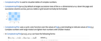
- ComplexArrayPlot 用于可视化复数表.
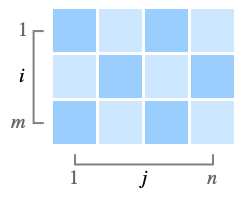
- ComplexArrayPlot[array] 默认情况下会安排 mn 维度数组 array 中连续行顺着页面往下排列,连续列顺着页面横向排列,就像普通的表格或网格的格式一样.
- ComplexArrayPlot 会在 Arg[zij] 的值上使用循环颜色函数,并使用明暗来表示 Abs[zij] 的值. 模数较大的复数比模数较小的复数更明亮.
- 在 ComplexArrayPlot[array] 中,array 可有如下格式:
-
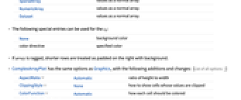
{{z11,z12,…,z1n},…,{zm1,zm2,…,zmn}} 值 zij SparseArray 以普通数组给出的值 NumericArray 以普通数组给出的值 Dataset 以普通数组给出的值 - 下列特殊条目可用于 zij:
-
None 背景颜色 颜色指令 指定颜色 - 若 array 长短不一,则较短的行会被看做是用背景在右边进行填充.
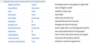
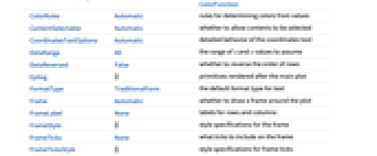
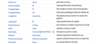
- ComplexArrayPlot 的选项与 Graphics 很像,有如下的添加和变化: [所有选项的列表]
-
AspectRatio Automatic 高与宽的比率 ClippingStyle None 如何显示数值被剪切的单元 ColorFunction Automatic 如何为每个单元上色 ColorFunctionScaling True 是否对 ColorFunction 的参数进行缩放 ColorRules Automatic 根据决定颜色的规则 DataRange All 假设的
和
值的范围DataReversed False 是否倒转行的顺序 Frame Automatic 是否为图形绘制边框 FrameLabel None 行和列的标签 FrameTicks None 边框中要包括的刻度 MaxPlotPoints Infinity 最多可以包含多少个点 Mesh False 是否绘制网格 MeshStyle GrayLevel[GoldenRatio-1] 网格使用的样式 PerformanceGoal $PerformanceGoal 优化的目标 PlotLegends None 数据集的图例 PlotRange All 绘制的值的范围 PlotTheme $PlotTheme 绘图的整体主题 TargetUnits Automatic 绘图中展示的单位 - ColorRules 给出的规则被应用于每个单元的
. 规则可以包括模式. - 如果没有应用 ColorRules 中的任何规则,则使用 ColorFunction 决定颜色.
- 如果使用默认设置 ColorRules->Automatic,则会使用明确的设置 ColorFunctioncfunc 而非 ColorRules.
- ColorFunction->{cfunc,sfunc} 使用 cfunc 生成基础颜色,并使用 sfunc 调整颜色以突出显示特征.
- sfunc 的可能的已命名设置包括:
-

Automatic 基于 Abs[z] 自动调整明暗 
"MaxAbs" Abs[z] 较大值的浅色调 
"LocalMaxAbs" Abs[z] 的上四分位数的的浅色调 
"GlobalAbs" 与 Abs[z] 从小到大的值对应的由暗到亮的色调 
"QuantileAbs" 基于 Abs[z] 的分位数的由暗到亮的色调 
"CyclicLogAbs" Log[Abs[z]] 的循环的由暗到亮的色调 
"CyclicArg" Arg[z] 的循环的由暗到亮的色调 
"CyclicLogAbsArg" Log[Abs[z]] 和 Arg[z] 的循环的色调 
"CyclicReImLogAbs" Re[z] 和 Im[z] 的暗色环,Log[Abs[z]] 的浅色环 
"ShiftedCyclicLogAbs" 超过特定阈值后的 Log[Abs[z]] 的循环的色调 
None 不改变色调 - 默认情况下,ColorFunction 中的函数由缩放版的 Re[z]、Im[z]、Abs[z] 和 Arg[z] 提供.
- 若某个特定单元格的颜色为 None,则该单元格用背景色进行渲染.
- 若未为某个特定的单元格决定颜色,则该单元格会以默认深红色渲染.
- 设置 DataReversed->True,则倒转行的顺序,这样行从底部到顶部排序,最后一行排在最上面.
- 设置 FrameTicks->Automatic,刻度通常放在四舍五入的整数位置,通常在 5 或 10 的倍数处.
- 设置 FrameTicks->All,刻度通常放在最小和最大的
和
处. - 在明确的 FrameTicks 设置下,刻度的坐标用于指代
和
. - PlotRange 可以有如下格式:
-
zmax 在 0 到 zmax 之间显示 Abs[zij] 的值 {zmin,zmax} 在 zmin 和 zmax 之间显示 Abs[zij] 的值 {rangei,rangej} 显示 zij 的值,其中 i 在 rangei 中且 j 在 rangej 中 {rangei,rangej,rangez} 显示 zij 的值,其中 i 在 rangei 中,j 在 rangej 中且 zij 在 rangez 中 - 数组指数范围为从 rangei 到 rangej,且可以有如下形式:
-
{min,max} 包括 min 和 max 之间的指数 All 包括所有指数 - PlotLegends 的一般设置包括:
-
None 没有图例 Automatic 自动决定图例 Placed[lspec,…] 明确图例的位置 - Mesh->True 在数组的每个单元格之间绘制网格线.
- Mesh->{mi,mj} 分别为
和
方向给出网格格式说明. - 默认设置 Frame->Automatic,边框仅在 Mesh->False 时绘制.
- 为了结合其他图形,使用数组元素
覆盖中心坐标位置为
,
的单位正方形. - 设置 DataRange->{{xmin,xmax},{ymin,ymax}} 说明连续单元格的中心应该处于 xmin 与 xmax 之间的水平方向和 ymin 与 ymax 之间的垂直方向的等距位置. 默认设置 DataReversed->False,
的中心在 {xmin,ymax}. - 默认设置 DataRange->All 且 DataReversed->False,数组元素
会被用来覆盖中心坐标位置为
,
的单位正方形.
所有选项的列表
范例
打开所有单元 关闭所有单元基本范例 (6)
ComplexArrayPlot[{{I, 1 + I, 1 - I}, {1, I / 2, 2 + 3I}}]ComplexArrayPlot[{{Black, Orange, 1 - I}, {1, I / 2, 2 + 3I}}]ComplexArrayPlot[{{I, 1 + I, 1 - I}, {1, I / 2, 2 + 3I}}, ColorRules -> {1 -> Blue, I -> Yellow}]ComplexArrayPlot[{{I, White, White}, {1, I / 2, 2 + 3I}}, Mesh -> True]ComplexArrayPlot[RandomComplex[{-1 - I, 1 + I}, {10, 20}]]ComplexArrayPlot[RandomComplex[{-1 - I, 1 + I}, {10, 20}], ColorFunction -> "BeachColors"]范围 (14)
数据 (8)
默认情况下,颜色会伴随着参数从
(青蓝)到
(红色)到
(青蓝)的变化而改变:
ComplexArrayPlot[{{-1 + I, I, 1 + I}, {-1, 0, 1}, {-1 - I, -I, 1 - I}}]ComplexArrayPlot[{{-2 + 2 I, -1 + 2 I, 2 I, 1 + 2 I, 2 + 2 I}, {-2 + I, -1 + I, I, 1 + I, 2 + I}, {-2, -1, 0, 1, 2}, {-2 - I, -1 - I, -I, 1 - I, 2 - I}, {-2 - 2 I, -1 - 2 I, -2 I, 1 - 2 I, 2 - 2 I}}]ComplexArrayPlot[{{X, Y, Z }, {, 0, 1}, {-1 - I, -I, Null}}]ComplexArrayPlot[{{Red, I, 1 + I}, {-1, Green, 1}, {-1 - I, -I, Blue}}]ComplexArrayPlot[{{-1 + I}, {-1, 0}, {-1 - I, -I, 1 - I}}]带有值 None 的单元格用背景色进行渲染:
ComplexArrayPlot[{{-1 + I, None, 1 + I}, {-1, None, 1}, {-1 - I, None, 1 - I}}]ComplexArrayPlot[SparseArray[{{x_, x_} -> 1 + I, ({x_, y_} /; Abs[x - y] < 3) :> RandomComplex[{-1 - I, 1 + I}]}, {10, 10}]]ComplexArrayPlot[RawArray["Complex64", {{-4.005686283111572 + 3.604153871536255*I,
4.635770320892334 - 1.1016300916671753*I, 1.9577208757400513 + 4.972633361816406*I,
3.506197690963745 - 0.33499598503112793*I, -2.474790334701538 - 3.884897232055664*I,
1 ... 9864978790283*I,
1.6527553796768188 + 0.20232297480106354*I, -1.0656682252883911 + 0.8207247257232666*I,
-1.9840965270996094 - 1.6973134279251099*I, 3.3480541706085205 - 4.883756160736084*I,
-4.373885631561279 + 2.1675751209259033*I}}]]演示 (6)
ComplexArrayPlot[{{-1 + I, I, 1 + I}, {-1, 0, 1}, {-1 - I, -I, 1 - I}}, Mesh -> True]ComplexArrayPlot[Reverse@Table[real + I imag, {imag, -10, 10}, {real, -10, 10}], PlotLegends -> Automatic]ComplexArrayPlot[Reverse@Table[real + I imag, {imag, -10, 10}, {real, -10, 10}], PlotLegends -> Automatic, ColorFunction -> {Automatic, None}]ComplexArrayPlot[Reverse@Table[real + I imag, {imag, -10, 10}, {real, -10, 10}], ColorFunction -> {"WatermelonColors", None}]使用阴影图示如 ComplexPlot:
ComplexArrayPlot[Reverse@Table[real + I imag, {imag, -40, 40}, {real, -40, 40}], ColorFunction -> "ShiftedCyclicLogAbs"]ComplexArrayPlot[Reverse@Table[real + I imag, {imag, -40, 40}, {real, -40, 40}], ColorFunction -> {"WatermelonColors", "ShiftedCyclicLogAbs"}]选项 (71)
AspectRatio (4)
ComplexArrayPlot[Mod[Array[Binomial, {32, 32}, 0], 1 + I]]ComplexArrayPlot[Mod[Array[Binomial, {32, 32}, 0], 1 + I], AspectRatio -> 1 / 2]设置 AspectRatio1 使高度与宽度相同:
ComplexArrayPlot[Mod[Array[Binomial, {32, 32}, 0], 1 + I], AspectRatio -> 1]AspectRatioFull 调整高度和宽度以紧密贴合其他构造:
plot = ComplexArrayPlot[Mod[Array[Binomial, {32, 32}, 0], 1 + I], AspectRatio -> Full];{Framed[Pane[plot, {50, 100}]], Framed[Pane[plot, {100, 100}]], Framed[Pane[plot, {100, 50}]]}Axes (4)
默认情况下,ComplexArrayPlot 使用边框而非轴:
ComplexArrayPlot[Mod[Array[Binomial, {32, 32}, 0], 1 + I]]ComplexArrayPlot[Mod[Array[Binomial, {32, 32}, 0], 1 + I], Frame -> False, Axes -> True]使用 AxesOrigin 可指定轴相交处:
ComplexArrayPlot[Mod[Array[Binomial, {32, 32}, 0], 1 + I], Frame -> False, Axes -> True, AxesOrigin -> {0, 0}]{ComplexArrayPlot[Mod[Array[Binomial, {32, 32}, 0], 1 + I], Frame -> False, Axes -> {True, False}], ComplexArrayPlot[Mod[Array[Binomial, {32, 32}, 0], 1 + I], Frame -> False, Axes -> {False, True}]}AxesLabel (3)
ComplexArrayPlot[Mod[Array[Binomial, {32, 32}, 0], 1 + I], Frame -> False, Axes -> True]ComplexArrayPlot[Mod[Array[Binomial, {32, 32}, 0], 1 + I], Frame -> False, Axes -> True, AxesLabel -> "Label"]ComplexArrayPlot[Mod[Array[Binomial, {32, 32}, 0], 1 + I], Frame -> False, Axes -> True, AxesLabel -> {"label 1", "Label 2"}]AxesOrigin (2)
AxesStyle (4)
ComplexArrayPlot[Mod[Array[Binomial, {32, 32}, 0], 1 + I], Frame -> False, Axes -> True, AxesStyle -> Red]ComplexArrayPlot[Mod[Array[Binomial, {32, 32}, 0], 1 + I], Frame -> False, Axes -> True, AxesStyle -> {{Thick, Red}, {Thick, Blue}}]ComplexArrayPlot[Mod[Array[Binomial, {32, 32}, 0], 1 + I], Frame -> False, Axes -> True, AxesStyle -> Green, TicksStyle -> Black]ComplexArrayPlot[Mod[Array[Binomial, {32, 32}, 0], 1 + I], Frame -> False, Axes -> True, AxesStyle -> Green, LabelStyle -> Black]Background (4)
Background 通常只可在边缘看到:
ComplexArrayPlot[{{0, 1, 2, 3}, {I, 1 + I, 2 + I, 3 + I}, {2 I, 1 + 2 I, 2 + 2 I, 3 + 2 I}}, Background -> Blue]只要明确输入了 None,就能直接看到背景颜色::
ComplexArrayPlot[{{None, 1, 2, 3}, {I, None, 2 + I, 3 + I}, {2 I, 1 + 2 I, None, 3 + 2 I}}, Background -> Blue]对于在绘图范围外的值,默认情况下也可以直接看到 Background:
ComplexArrayPlot[{{0, 1, 2, 3}, {I, 1 + I, 2 + I, 3 + I}, {2 I, 1 + 2 I, 2 + 2 I, 3 + 2 I}}, Background -> Blue, PlotRange -> {1, 3}]ClippingStyle 覆写背景颜色:
ComplexArrayPlot[{{0, 1, 2, 3}, {I, 1 + I, 2 + I, 3 + I}, {2 I, 1 + 2 I, 2 + 2 I, 3 + 2 I}}, Background -> Blue, PlotRange -> {1, 3}, ClippingStyle -> {White, Black}]ClippingStyle (3)
ComplexArrayPlot[Table[(real + I imag)^2 + 1, {imag, -5, 5}, {real, -5, 5}], PlotRange -> {3, 20}]ComplexArrayPlot[Table[(real + I imag)^2 + 1, {imag, -5, 5}, {real, -5, 5}], PlotRange -> {3, 20}, ClippingStyle -> Red]ComplexArrayPlot[Table[(real + I imag)^2 + 1, {imag, -5, 5}, {real, -5, 5}], PlotRange -> {3, 20}, ClippingStyle -> {Black, Red}]ColorFunction (9)
默认情况下,复数
的值由 Arg[z] 上色并由 Abs[z] 添加阴影:
ComplexArrayPlot[Table[(real + I imag)^4 + 1, {imag, -20, 20}, {real, -20, 20}]]根据 Abs[z] 关闭阴影功能:
ComplexArrayPlot[Table[(real + I imag)^4 + 1, {imag, -20, 20}, {real, -20, 20}], ColorFunction -> None]根据 Hue 将从 0 到 1 的模数值映射到颜色上:
ComplexArrayPlot[Table[(real + I imag)^4 + 1, {imag, -20, 20}, {real, -20, 20}], ColorFunction -> Hue]ComplexArrayPlot[Table[(real + I imag)^4 + 1, {imag, -20, 20}, {real, -20, 20}], ColorFunction -> (GrayLevel[#4]&)]使用 ColorData 中有名称的渐变颜色:
ComplexArrayPlot[Table[(real + I imag)^4 + 1, {imag, -20, 20}, {real, -20, 20}], ColorFunction -> "StarryNightColors"]ComplexArrayPlot[Table[(real + I imag)^4 + 1, {imag, -50, 50}, {real, -50, 50}], ColorFunction -> "ShiftedCyclicLogAbs"]ComplexArrayPlot[Table[(real + I imag)^4 + 1, {imag, -50, 50}, {real, -50, 50}], ColorFunction -> {"DarkRainbow", "CyclicArg"}]设置 ColorFunctionScalingTrue,则值会首先被缩放至 0 到 1 之间:
ComplexArrayPlot[Table[(real + I imag)^4 + 1, {imag, -50, 50}, {real, -50, 50}], ColorFunction -> "DarkRainbow", ColorFunctionScaling -> False]使用通过 Re[z]、Im[z]、Abs[z] 或 Arg[z] 为复值
上色的颜色函数:
ComplexArrayPlot[Table[(real + I imag)^4 + 1, {imag, -50, 50}, {real, -50, 50}], ColorFunction -> Function[{re, im, abs, arg}, Blend[{Red, Green}, abs]]]ColorFunctionScaling (3)
默认情况下,在应用颜色函数前会将值缩放至 0 到 1 之间:
ComplexArrayPlot[Table[(real + I imag)^4 + 1, {imag, -20, 20}, {real, -20, 20}], ColorFunctionScaling -> True, PlotLegends -> Automatic]ComplexArrayPlot[Table[(real + I imag)^4 + 1, {imag, -20, 20}, {real, -20, 20}], ColorFunctionScaling -> False, PlotLegends -> Automatic]ComplexArrayPlot[Table[(real + I imag)^4 + 1, {imag, -50, 50}, {real, -50, 50}], ColorFunction -> "DarkRainbow", ColorFunctionScaling -> False, PlotLegends -> Automatic]ColorRules (6)
ComplexArrayPlot[Table[Gamma[real + I imag], {imag, -5, 5}, {real, -5, 5}], ColorRules -> {1 -> Black, Gamma[3I] -> White, Gamma[-3I] -> White}]realQ[z_] := Re[z] == zComplexArrayPlot[Table[Gamma[real + I imag], {imag, -5, 5}, {real, -5, 5}], ColorRules -> {_ ? realQ -> Black}]如果不应用任何颜色规则的话,则会使用 ColorFunction:
imaginaryQ[z_] := I Im[z] == zComplexArrayPlot[Table[Gamma[real + I imag], {imag, -5, 5}, {real, -5, 5}], ColorRules -> {_ ? imaginaryQ -> Black}]ComplexArrayPlot[Transpose[Permutations[{a, b, c}]], ColorRules -> {a -> Red, b -> Yellow, c -> Blue}, Mesh -> True]realQ[z_] := Re[z] == zComplexArrayPlot[Table[Gamma[real + I imag], {imag, -2, 2}, {real, -2, 2}], ColorRules -> {_ ? realQ -> Black, _ -> Yellow}]realQ[z_] := Re[z] == zComplexArrayPlot[Table[Gamma[real + I imag], {imag, -5, 5}, {real, -5, 5}], ColorRules -> {1 -> White, _ ? realQ -> Black}]DataRange (5)
ComplexArrayPlot[Table[Gamma[real + I imag], {imag, 0, 3}, {real, 0, 5}], FrameTicks -> Automatic]ComplexArrayPlot[Table[Gamma[real + I imag], {imag, 0, 3}, {real, 0, 5}], FrameTicks -> Automatic, DataRange -> {{0, 5}, {0, 3}}]ComplexArrayPlot[Table[Gamma[real + I imag], {imag, 0, 3}, {real, 0, 5}], FrameTicks -> Automatic, DataRange -> {1 + 2I, 6 + 5I}]ComplexArrayPlot[Table[Gamma[real + I imag], {imag, 0, 3}, {real, 0, 5}], FrameTicks -> Automatic, DataRange -> {0, All}]ComplexArrayPlot[Table[Gamma[real + I imag], {imag, 0, 3}, {real, 0, 5}], FrameTicks -> Automatic, DataRange -> {All, 0}]DataReversed (4)
ComplexArrayPlot[Table[ArcCos[real + I imag], {imag, 0, 3}, {real, 0, 5}], DataReversed -> True]ComplexArrayPlot[Table[ArcCos[real + I imag], {imag, 0, 3}, {real, 0, 5}], FrameTicks -> Automatic, DataReversed -> True]ComplexArrayPlot[Table[ArcCos[real + I imag], {imag, 0, 3}, {real, 0, 5}], FrameTicks -> Automatic, DataReversed -> {True, True}]ComplexArrayPlot[Table[ArcCos[real + I imag], {imag, 0, 3}, {real, 0, 5}], FrameTicks -> Automatic, DataReversed -> {False, True}]Epilog (3)
使用 Epilog 可叠加在其他图形上:
ComplexArrayPlot[RandomComplex[{-1 - I, 1 + I}, {5, 5}], Epilog -> Disk[]]ComplexArrayPlot[RandomComplex[{-1 - I, 1 + I}, {5, 5}], Epilog -> Disk[{3, 3}, 1]]ComplexArrayPlot[RandomComplex[{-1 - I, 1 + I}, {5, 5}], Epilog -> {Opacity[0.5], Disk[{3, 3}, 1]}]MaxPlotPoints (1)
使用 MaxPlotPoints 可以在每个方向上明确限制绘制的元素的数量:
ComplexArrayPlot[Partition[Table[PowerMod[1 + 3I, k, 7], {k, 0, 2^14 - 1}], 2^7]]ComplexArrayPlot[Partition[Table[PowerMod[1 + 3I, k, 7], {k, 0, 2^14 - 1}], 2^7], MaxPlotPoints -> 50]Mesh (4)
ComplexArrayPlot[Partition[Table[k Exp[2π I k / 32], {k, 0, 31}], 8], Mesh -> All]ComplexArrayPlot[Partition[Table[k Exp[2π I k / 32], {k, 0, 31}], 8], Mesh -> {1, 3}]ComplexArrayPlot[Partition[Table[k Exp[2π I k / 32], {k, 0, 31}], 8], Mesh -> {None, Range[4]}]ComplexArrayPlot[Partition[Table[k Exp[2π I k / 32], {k, 0, 31}], 8], Mesh -> {None, Table[{i, GrayLevel[i / 8]}, {i, 0, 8}]}]MeshStyle (2)
ComplexArrayPlot[Partition[Table[k Exp[2π I k / 32], {k, 0, 31}], 8], Mesh -> All, MeshStyle -> Directive[Black, Thick]]ComplexArrayPlot[Partition[Table[k Exp[2π I k / 32], {k, 0, 31}], 8], Mesh -> All, MeshStyle -> {Directive[Black, Thick], White}]PlotLegends (5)
ComplexArrayPlot[Array[(#1 + I #2)^3&, {10, 10}, 0]]ComplexArrayPlot[Array[(#1 + I #2)^3&, {10, 10}, 0], PlotLegends -> Automatic]PlotLegends 自动识别有名称的 ColorFunction:
ComplexArrayPlot[Array[(#1 + I #2)^3&, {10, 10}, 0], PlotLegends -> Automatic, ColorFunction -> {"TemperatureMap", "CyclicLogAbsArg"}]PlotLegends 不会识别用户自定义的 ColorFunction,但是用户仍然可以构建合适的图例:
Legended[ComplexArrayPlot[Array[(#1 + I #2)^3&, {10, 10}, 0], PlotLegends -> Automatic, ColorFunction -> {(RGBColor[#4, 0.5, 0]&), None}], BarLegend[{(RGBColor[#, 0.5, 0]&), {-π, π}}]]使用 Placed 改变图例的位置:
ComplexArrayPlot[Array[(#1 + I #2)^3&, {10, 10}, 0], PlotLegends -> Placed[Automatic, Below]]PlotRange (4)
ComplexArrayPlot[Array[I#1Sin[#1 + #2]&, {5, 15}]]绘制
的值,其中 1≤Abs[z]≤2:
ComplexArrayPlot[Array[I#1Sin[#1 + #2]&, {5, 15}], PlotRange -> {1, 2}]绘制
的值,其中 Abs[z]≤2:
ComplexArrayPlot[Array[I#1Sin[#1 + #2]&, {5, 15}], PlotRange -> 2]PlotRange 的前两个条目指定了要包括的行和列的范围:
ComplexArrayPlot[Array[I#1Sin[#1 + #2]&, {5, 15}], PlotRange -> {{2, 4}, All, {0, 2}}]应用 (18)
傅立叶变换 (6)
n = 16;
{f1, f2} = {3, 5};
data = Table[Sin[(2π f1 x/n)]Sin[(2π f2 y/n)], {x, 0, n - 1}, {y, 0, n - 1}];fft = Chop[Fourier[data]];展示原始数据和其傅立叶变换. 在第二个绘图中,第四行和第六列(从左上角开始数)的浅色方块告诉我们对应的频率分别为 3 和 5:
{ArrayPlot[data], ComplexArrayPlot[fft, Mesh -> All]}data2 = Table[Sin[(2π f1 x/n)]Sin[(2π f2 y/n)] + 3Sin[(2π f2 x/n)] - 8Sin[(2π f1 y/n)], {x, 0, n - 1}, {y, 0, n - 1}];ComplexArrayPlot[Chop@Fourier[data2], Mesh -> All]data = 1 - ImageData[Binarize@Rasterize["I"]];{ArrayPlot[data], ComplexArrayPlot[Fourier[data]]}使用 ColorRules 为傅立叶变换设置阈值:
data = ImageData[ImageResize[ColorConvert[[image], "Grayscale"], {64, 64}]];{ArrayPlot[data], ComplexArrayPlot[Fourier[data], ColorRules -> {_ ? (Abs[#] < 0.2&) -> Black}, ColorFunction -> None]}data = ImageData[Binarize[[image]]];ComplexArrayPlot[Take[#, 34]& /@ Take[Fourier[data], 34], ColorFunction -> "BlueGreenYellow", PlotLegends -> Automatic]data = Quiet@Table[((2BesselJ[1, Sqrt[x^2 + y^2]]/Sqrt[x^2 + y^2]))^2, {x, -30, 30}, {y, -30, 30}] /. Indeterminate -> 1;{ArrayPlot[Log@data], ComplexArrayPlot[Fourier[data]]}data = CrossMatrix[10];
data2 = RotateLeft[#, 10]& /@ data;绘制了傅立叶变换的幅度,但这并未显示可能有用的相位信息. 观察中间的绘图中其他的信息:
{ArrayPlot[data, PlotLabel -> "Original Data"], ComplexArrayPlot[Fourier[data], PlotLabel -> "Fourier Transform"], ArrayPlot[Abs[Fourier@data], PlotLabel -> "|Fourier Transform|"]}注意傅立叶变换中 ComplexArrayPlot 的变化和 ArrayPlot 没有变化:
{ArrayPlot[data2, PlotLabel -> "Original Data"], ComplexArrayPlot[Fourier[data2], PlotLabel -> "Fourier Transform"], ArrayPlot[Abs[Fourier@data2], PlotLabel -> "|Fourier Transform|"]}矩阵表示 (3)
m = SparseArray[{{30, _} -> 1, {_, 30} -> -1, {j_, k_} /; Abs[j - k] ≤ 1 :> Exp[2π I k / 50]}, {50, 50}];ComplexArrayPlot[m, ColorRules -> {0 -> Black}, ColorFunction -> None]m = RandomComplex[{-1 - I, 1 + I}, {8, 8}];ComplexArrayPlot[m]p = Transpose[Eigenvectors[m]];ComplexArrayPlot[Chop[Inverse[p].m.p], ColorRules -> {0 -> White}]{q, r} = QRDecomposition[m];ComplexArrayPlot /@ {q, r}ComplexArrayPlot[KroneckerProduct[PauliMatrix[#[[1]]], PauliMatrix[#[[2]]]], ColorRules -> {0 -> White}, ColorFunction -> None, PlotLabel -> Subscript[σ, #[[1]]]⊗Subscript[σ, #[[2]]]]& /@ Subsets[Range[3], {2}]ComplexArrayPlot[KroneckerProduct[PauliMatrix[#[[2]]], PauliMatrix[#[[1]]]], ColorRules -> {0 -> White}, ColorFunction -> None, PlotLabel -> Subscript[σ, #[[2]]]⊗Subscript[σ, #[[1]]]]& /@ Subsets[Range[3], {2}]吸引盆 (2)
f[z_] := z^3 - 1newtonMapf = Compile[{{z, _Complex}}, Evaluate[z - (f[z]/f'[z])]];rootsf = Quiet@Reverse[Table[Nest[newtonMapf, 1.0x + I y, 100], {y, -1, 1, 0.01}, {x, -1, 1, 0.01}]];//TimingComplexArrayPlot[rootsf, ColorFunction -> None, PlotLegends -> SwatchLegend[{LABColor[0.5487947278149338, 0.629271353261171, 0.4277070533203531], LABColor[0.740301849178597, -0.5551479480848852, 0.5722452976336212], LABColor[0.4836757194298422, 0.3968716772040611, -0.7197934077503745]}, {1, Exp[2π I / 3], Exp[-2π I / 3]}]]g[z_] := Sin[z^3 - 1]newtonMapg = Compile[{{z, _Complex}}, Evaluate[z - (g[z]/g'[z])]];ComplexListPlot[Table[z /. NSolve[z^3 - 1 == n π, z], {n, 0, 10}]]rootsg = Quiet@Reverse[Table[Nest[newtonMapg, 1.0x + I y, 100], {y, -1, 1, 0.005}, {x, -1, 1, 0.005}]];ComplexArrayPlot[rootsg, ColorFunction -> "CyclicLogAbs"]f[z_] := z^3 - 1halleyMapf = Compile[{{z, _Complex}}, Evaluate[z - (2f[z] Derivative[1][f][z]/2Derivative[1][f][z]^2 - f[z] Derivative[2][f][z])]];rootsf = Quiet@Table[Nest[halleyMapf, 1.0x + I y, 10], {y, -2, 2, 0.01}, {x, -2, 2, 0.01}];ComplexArrayPlot[rootsf, ColorFunction -> None, PlotLegends -> SwatchLegend[{LABColor[0.5487947278149338, 0.629271353261171, 0.4277070533203531], LABColor[0.740301849178597, -0.5551479480848852, 0.5722452976336212], LABColor[0.4836757194298422, 0.3968716772040611, -0.7197934077503745]}, {1, Exp[2π I / 3], Exp[-2π I / 3]}]]矩阵光谱 (2)
eigs = Table[Eigenvalues[{{1, a}, {1, b}}], {b, -10, 10}, {a, -10, 10}];{ComplexArrayPlot[Map[First, eigs, {2}]],
ComplexArrayPlot[Map[Last, eigs, {2}]]}m = (| | | | |
| - | ----- | - | - |
| 0 | 1 | 0 | 0 |
| 0 | 0 | 1 | 0 |
| 0 | 0 | 0 | 1 |
| 0 | 1 - I | I | 0 |);Eigenvalues[m]矩阵
的 ϵ-伪谱是复平面中
值的合集,该复平面中 (m-λ I)-1 的范数大于
. 为 ϵ=1,1/2,1/4,1/8,1/16,1/32 绘制ϵ-伪谱,并注意白点处的特征值:
ContourPlot[Norm[Inverse[1.0m - (x + I y) IdentityMatrix[4]], 2], {x, -2, 2}, {y, -2, 2}, Contours -> {1, 2, 4, 8, 16, 32}, PlotRange -> {0, 64}, ColorFunction -> "CMYKColors"]如果使用最大特征值而非 (m-λ I)-1 的范数,则可以添加参数信息:
data = Reverse@Table[First@Eigenvalues[Quiet@Inverse[m - (x + I y) IdentityMatrix[4, SparseArray]], 1], {y, -2, 2, 0.01}, {x, -2, 2, 0.01}];
ComplexArrayPlot[data]t = ToeplitzMatrix[PadRight[{1, -1}, 10], PadRight[{1, 1, 1, 1}, 10]];
MatrixForm[t]data = Reverse@Table[First@Eigenvalues[Inverse[t - (x + I y) IdentityMatrix[10, SparseArray]], 1], {y, -2.5, 2.5, 0.01}, {x, -2.5, 2.5, 0.01}];//Timing
ComplexArrayPlot[data, ColorFunction -> "QuantileAbs"]mat = ExampleData[{"Matrix", "WEST0067"}];data = Table[First@Eigenvalues[Inverse[mat - (x + I y) IdentityMatrix[Length[mat], SparseArray]], 1], {y, -2, 2, 0.05}, {x, -2, 2, 0.05}];
ComplexArrayPlot[data, ColorFunction -> {"DarkRainbow", "GlobalAbs"}]迭代系统 (3)
ComplexArrayPlot[CellularAutomaton[{{a_, b_} -> a b}, {{Exp[2π I / 3]}, 1}, 3^4 - 1], ColorFunction -> None, ColorRules -> {1 -> White}]ComplexArrayPlot[CellularAutomaton[{{a_, b_} -> a b}, {{Exp[π I / 4]}, 1}, 2^8 - 1], ColorFunction -> None, ColorRules -> {1 -> White}]ComplexArrayPlot[CellularAutomaton[{{a_, b_} -> a - b}, {{Exp[π I / 4]}, 1}, 20], ColorFunction -> None, ColorRules -> {1 -> Black, 0 -> White}]c = 1.0 + I;
data = NestList[#^2 + c&, 0.0, 50];ComplexArrayPlot[Partition[data, 10]]c = (1.0 + I/3);
data = NestList[#^2 + c&, 0.0, 50];ComplexArrayPlot[Partition[data, 10]]Clear[c];
c = c /. Solve[Nest[#^2 + c&, 0, 7] == 0, c][[20]];
data = NestList[#^2 + c&, 0.0, 50]//Chop;ComplexArrayPlot[Partition[data, 10]]设
是复数系数
的对数函数. 思考在
时数列
,
. 在未为
设定边界的情况下计算
的近似值,并可视化该区域:
a = Reverse@Table[Quiet@FixedPoint[(c1 + I c2)#(1 - #)&, 1.1, 20], {c2, -2, 2, 0.02}, {c1, -2, 2, 0.02}];//Timing
a = a /. {z_ ? NumericQ :> If[Abs[z] < 1000, z, 0]};
Quiet@ComplexArrayPlot[a, ColorRules -> {0 -> Black}]其他 (2)
gaussianPrimeQ[c_] := PrimeQ[c, GaussianIntegers -> True]n = 20;
pts = Outer[#1 + I #2&, Range[-n, n], Range[-n, n]];
ComplexArrayPlot[pts, ColorRules -> {_ ? gaussianPrimeQ -> Black}, DataRange -> {{-n, n}, {-n, n}}, FrameTicks -> All]n = 32;
mat = Table[(1/Sqrt[n])Exp[2.0π I j k / n], {j, 0, n - 1}, {k, 0, n - 1}];ComplexArrayPlot[mat, ColorFunction -> None]ComplexArrayPlot[Chop@mat, ColorRules -> {z_ /; Re[z] == 0 -> Gray, z_ /; Im[z] == 0 -> Black}]属性和关系 (5)
ComplexArrayPlot 通过参数为复值上色,并通过像 ComplexPlot 这样的模数添加阴影:
f[z_] := I Sin[z^2 + 1]data = Reverse@Table[f[x + I y], {y, -2, 2, 0.05}, {x, -2, 2, 0.05}];{ComplexArrayPlot[Reverse@Table[f[x + I y], {y, -2, 2, 0.05}, {x, -2, 2, 0.05}]], ComplexPlot[f[z], {z, -2 - 2I, 2 + 2I}]}ComplexArrayPlot 类似应用于复值参数的 ArrayPlot 和 MatrixPlot:
data = Table[Sin[x + I y], {y, -2, 2, 0.25}, {x, -2, 2, 0.25}];{ComplexArrayPlot[data], ArrayPlot[Arg[data], ColorFunction -> (Hue[# + 0.5]&)], MatrixPlot[Arg[data], ColorFunction -> (Hue[# + 0.5]&)]}Grid 排列元素的方法与 ComplexArrayPlot 一样:
data = {{0, Exp[I π / 4], I, Exp[3I π / 4]}, {-1, Exp[-3I π / 4], -I, Exp[-I π / 4]}};Grid[data]ComplexArrayPlot[data, PlotLegends -> Automatic, ColorFunction -> None]Raster 将与 ComplexArrayPlot 有关的元素上下倒转排列:
data = {{0, Exp[I π / 4], I, Exp[3I π / 4]}, {-1, Exp[-3I π / 4], -I, Exp[-I π / 4]}};{ComplexArrayPlot[data, ColorFunction -> {(GrayLevel[#4]&), None}], Graphics[Raster[(Arg[data] + π/2π)]]}ArrayPlot3D 可用于数据的三维数组:
ArrayPlot3D[RandomInteger[1, {3, 4, 5}]]相关指南
-
▪
- 复数可视化
文本
Wolfram Research (2020),ComplexArrayPlot,Wolfram 语言函数,https://reference.wolfram.com/language/ref/ComplexArrayPlot.html.
CMS
Wolfram 语言. 2020. "ComplexArrayPlot." Wolfram 语言与系统参考资料中心. Wolfram Research. https://reference.wolfram.com/language/ref/ComplexArrayPlot.html.
APA
Wolfram 语言. (2020). ComplexArrayPlot. Wolfram 语言与系统参考资料中心. 追溯自 https://reference.wolfram.com/language/ref/ComplexArrayPlot.html 年
BibTeX
@misc{reference.wolfram_2026_complexarrayplot, author="Wolfram Research", title="{ComplexArrayPlot}", year="2020", howpublished="\url{https://reference.wolfram.com/language/ref/ComplexArrayPlot.html}", note=[Accessed: 10-September-2026]}
BibLaTeX
@online{reference.wolfram_2026_complexarrayplot, organization={Wolfram Research}, title={ComplexArrayPlot}, year={2020}, url={https://reference.wolfram.com/language/ref/ComplexArrayPlot.html}, note=[Accessed: 10-September-2026]}