


RegionPlot3D
RegionPlot3D[pred,{x,xmin,xmax},{y,ymin,ymax},{z,zmin,zmax}]
makes a plot showing the three-dimensional region in which pred is True.
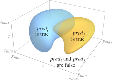
RegionPlot3D[{pred1,pred2,…},…]
plots several regions corresponding to the predi.
Details and Options
- The predicate pred can be any logical combination of inequalities.
- The region plotted by RegionPlot3D can contain disconnected parts.
- RegionPlot3D treats the variables x, y and z as local, effectively using Block.
- RegionPlot3D has attribute HoldAll and evaluates pred after assigning numerical values to x, y and z. In some cases, it may be more efficient to use Evaluate to evaluate pred symbolically first.
- RegionPlot3D has the same options as Graphics3D, with the following additions and changes: [List of all options]
-
Axes True whether to draw axes BoundaryStyle Automatic how to draw boundaries of regions BoxRatios {1,1,1} bounding 3D box ratios ColorFunction Automatic how to color surfaces ColorFunctionScaling True whether to scale arguments to ColorFunction EvaluationMonitor None expression to evaluate at every function evaluation MaxRecursion Automatic the maximum number of recursive subdivisions allowed Mesh Automatic how many mesh lines in each direction to draw MeshFunctions {#1&,#2&,#3&} how to determine the placement of mesh lines MeshShading None how to shade regions between mesh lines MeshStyle Automatic the style for mesh lines Method Automatic the method to use for refining surfaces NormalsFunction Automatic how to determine effective surface normals PerformanceGoal $PerformanceGoal aspects of performance to try to optimize PlotLegends None legends for surfaces PlotPoints Automatic the initial number of sample points in each direction PlotRange Full the range of values to include in the plot PlotStyle Automatic graphics directives for the style of the surface of each region PlotTheme $PlotTheme overall theme for the plot ScalingFunctions None how to scale individual coordinates TextureCoordinateFunction Automatic how to determine texture coordinates TextureCoordinateScaling True whether to scale arguments to TextureCoordinateFunction WorkingPrecision MachinePrecision the precision used in internal computations - RegionPlot3D initially evaluates pred at a 3D grid of equally spaced sample points specified by PlotPoints. Then it uses an adaptive algorithm to subdivide at most MaxRecursion times, attempting to find the boundaries of all regions in which pred is True.
- You should realize that since it uses only a finite number of sample points, it is possible for RegionPlot3D to miss regions in which pred is True. To check your results, you should try increasing the settings for PlotPoints and MaxRecursion.
- With the default setting PlotRangeFull, RegionPlot3D will explicitly include the full ranges xmin to xmax, etc.
- With MeshAll, RegionPlot3D will explicitly draw mesh lines to indicate the subdivisions it used to find each region.
- RegionPlot3D can in general only find regions of positive measure; it cannot find regions that are just lines or points.
- The arguments supplied to functions in MeshFunctions are x, y, and z. Functions in ColorFunction and TextureCoordinateFunction are by default supplied with scaled versions of these arguments.
- RegionPlot3D returns Graphics3D[GraphicsComplex[data]].
- Possible settings for ScalingFunctions include:
-
{sx,sy,sz} scale x, y and z axes - Common built-in scaling functions s include:
-
"Log" 
log scale with automatic tick labeling "Log10" 
base-10 log scale with powers of 10 for ticks "SignedLog" 
log-like scale that includes 0 and negative numbers "Reverse" 
reverse the coordinate direction
List of all options
Examples
open all close allBasic Examples (6)
RegionPlot3D[x ^ 2 + y ^ 3 - z ^ 2 > 0, {x, -2, 2}, {y, -2, 2}, {z, -2, 2}]RegionPlot3D[{x + y + z < -2, x + y + z > 2}, {x, -2, 2}, {y, -2, 2}, {z, -2, 2}]Plot 3D regions defined by logical combinations of inequalities:
RegionPlot3D[x ^ 2 + y ^ 2 + z ^ 2 < 1 && x ^ 2 + y ^ 2 < z ^ 2, {x, -1, 1}, {y, -1, 1}, {z, -1, 1}, PlotPoints -> 35, PlotRange -> All]Use simple styling of region boundaries:
RegionPlot3D[x y z < 1, {x, -5, 5}, {y, -5, 5}, {z, -5, 5}, PlotStyle -> Directive[Yellow, Opacity[0.5]], Mesh -> None]RegionPlot3D[Sphere[]]Plot a region-constrained function:
RegionPlot3D[Sin[x] Cos[y] + Sin[y] Cos[z] + Sin[z] Cos[x] > 0, {x, y, z}∈ Ball[{0, 0, 0}, 10], PlotPoints -> 60, Mesh -> None, PlotStyle -> Directive[Orange, Specularity[White, 50], Opacity[0.9]], Boxed -> False, Axes -> False]Scope (12)
Sampling (3)
Areas where the function is not True are excluded:
RegionPlot3D[x ^ 2 + y ^ 2 ≤ z ^ 2 + 1, {x, -2, 2}, {y, -2, 2}, {z, -2, 2}]Use logical combinations of regions:
RegionPlot3D[x ^ 2 + y ^ 2 + z ^ 2 ≤ 4 && y ^ 2 + z ^ 2 ≤ 3, {x, -2, 2}, {y, -2, 2}, {z, -2, 2}]Regions do not have to be connected:
RegionPlot3D[x y z ≥ 1, {x, -2, 2}, {y, -2, 2}, {z, -2, 2}]Presentation (9)
Provide an explicit PlotStyle for the region:
RegionPlot3D[(x ^ 2 + y ^ 2 + z ^ 2) - (x ^ 4 + y ^ 4 + z ^ 4) > 1 / 2, {x, -1, 1}, {y, -1, 1}, {z, -1, 1}, PlotStyle -> Orange]Specify styles for each region:
RegionPlot3D[{x ^ 2 + y ^ 2 ≤ 1, x ^ 2 + z ^ 2 ≤ 1, y ^ 2 + z ^ 2 ≤ 1}, {x, -2, 2}, {y, -2, 2}, {z, -2, 2}, PlotStyle -> {Red, Orange, Yellow}, Mesh -> None]RegionPlot3D[z ^ 2 - 1 <= x ^ 2 + y ^ 2 ≤ z ^ 2 + 1, {x, -2.3, 2.3}, {y, -2.3, 2.3}, {z, -2, 2}, PlotLabel -> z ^ 2 - 1 <= x ^ 2 + y ^ 2 ≤ z ^ 2 + 1, PlotStyle -> Directive[Specularity[White, 10], Opacity[0.85], Purple], PlotPoints -> 20, AxesLabel -> Automatic, AxesEdge -> {{-1, 0}, {1, 0}, {-1, 0}}, Mesh -> False]RegionPlot3D[x ^ 2 + y ^ 2 + z ^ 2 ≤ 4 && y ^ 2 + z ^ 2 ≤ 2, {x, -2, 2}, {y, -2, 2}, {z, -2, 2}, Mesh -> 9, MeshFunctions -> {#2&, #3&}, MeshStyle -> Red]Style the areas between mesh lines:
RegionPlot3D[x y z ≥ -1, {x, -5, 5}, {y, -5, 5}, {z, -5, 5}, Mesh -> 8, MeshFunctions -> {Function[{x, y, z}, Norm[{x, y, z}]]}, MeshShading -> {Directive[Yellow, Opacity[0.4]], FaceForm[Cyan, Red]}]Color the region with an overlay density:
RegionPlot3D[x y z ≥ -8, {x, -5, 5}, {y, -5, 5}, {z, -5, 5}, ColorFunction -> Function[{x, y, z}, Hue[Rescale[x y z, {1, 5 ^ 3}]]], ColorFunctionScaling -> False, Mesh -> None]Use a theme with simple ticks in a bright color scheme:
RegionPlot3D[z ^ 2 - 1 <= x ^ 2 + y ^ 2 ≤ z ^ 2 + 1, {x, -2.3, 2.3}, {y, -2.3, 2.3}, {z, -2, 2}, PlotTheme -> "Business"]RegionPlot3D[z ^ 2 - 1 <= x ^ 2 + y ^ 2 ≤ z ^ 2 + 1, {x, -2.3, 2.3}, {y, -2.3, 2.3}, {z, -2, 2}, PlotTheme -> "Monochrome"]Apply a log scale to the z axis:
RegionPlot3D[x ^ 2 + y ^ 2 < z^2, {x, -10, 10}, {y, -10, 10}, {z, 0, 10}, ScalingFunctions -> {None, None, "Log"}]Options (82)
Axes (3)
By default, Axes are drawn:
RegionPlot3D[x ^ 2 + (2y) ^ 2 + (3z) ^ 2 ≤ 1, {x, -1, 1}, {y, -1 / 2, 1 / 2}, {z, -1 / 3, 1 / 3}]Use AxesFalse to turn off axes:
RegionPlot3D[x ^ 2 + (2y) ^ 2 + (3z) ^ 2 ≤ 1, {x, -1, 1}, {y, -1 / 2, 1 / 2}, {z, -1 / 3, 1 / 3}, Axes -> False]Turn each axis on individually:
{RegionPlot3D[x ^ 2 + (2y) ^ 2 + (3z) ^ 2 ≤ 1, {x, -1, 1}, {y, -1 / 2, 1 / 2}, {z, -1 / 3, 1 / 3}, Axes -> {True, False, False}], RegionPlot3D[x ^ 2 + (2y) ^ 2 + (3z) ^ 2 ≤ 1, {x, -1, 1}, {y, -1 / 2, 1 / 2}, {z, -1 / 3, 1 / 3}, Axes -> {False, True, False}], RegionPlot3D[x ^ 2 + (2y) ^ 2 + (3z) ^ 2 ≤ 1, {x, -1, 1}, {y, -1 / 2, 1 / 2}, {z, -1 / 3, 1 / 3}, Axes -> {False, False, True}]}AxesLabel (4)
No axes labels are drawn by default:
RegionPlot3D[x y z < 1, {x, -5, 5}, {y, -5, 5}, {z, -5, 5}]RegionPlot3D[x y z < 1, {x, -5, 5}, {y, -5, 5}, {z, -5, 5}, AxesLabel -> z]RegionPlot3D[x y z < 1, {x, -5, 5}, {y, -5, 5}, {z, -5, 5}, AxesLabel -> {X, Y, Z}]Use labels based on variables specified in RegionPlot3D:
RegionPlot3D[x y z < 1, {x, -5, 5}, {y, -5, 5}, {z, -5, 5}, AxesLabel -> Automatic]AxesOrigin (2)
AxesStyle (3)
Change the style for the axes:
RegionPlot3D[x ^ 2 + (2y) ^ 2 + (3z) ^ 2 ≤ 1, {x, -1, 1}, {y, -1 / 2, 1 / 2}, {z, -1 / 3, 1 / 3}, AxesStyle -> Red]Specify the style of each axis:
RegionPlot3D[x ^ 2 + (2y) ^ 2 + (3z) ^ 2 ≤ 1, {x, -1, 1}, {y, -1 / 2, 1 / 2}, {z, -1 / 3, 1 / 3}, AxesStyle -> {{Thick, Brown}, {Thick, Blue}, {Thick, Green}}]Use different styles for the ticks and the axes:
RegionPlot3D[x ^ 2 + (2y) ^ 2 + (3z) ^ 2 ≤ 1, {x, -1, 1}, {y, -1 / 2, 1 / 2}, {z, -1 / 3, 1 / 3}, AxesStyle -> Green, TicksStyle -> StandardBlue]BoundaryStyle (3)
Boundary lines are black by default:
RegionPlot3D[x y z ≥ 1, {x, -5, 5}, {y, -5, 5}, {z, -5, 5}, Mesh -> None]Use None to not draw any boundary lines:
RegionPlot3D[x y z ≥ 1, {x, -5, 5}, {y, -5, 5}, {z, -5, 5}, BoundaryStyle -> None, Mesh -> None]RegionPlot3D[x y z ≥ 1, {x, -5, 5}, {y, -5, 5}, {z, -5, 5}, BoundaryStyle -> Red, Mesh -> None]BoxRatios (2)
Regions are shown in a cube by default:
RegionPlot3D[x ^ 2 + (2y) ^ 2 + (3z) ^ 2 ≤ 1, {x, -1, 1}, {y, -1 / 2, 1 / 2}, {z, -1 / 3, 1 / 3}]Use the natural scale of the region:
RegionPlot3D[x ^ 2 + (2y) ^ 2 + (3z) ^ 2 ≤ 1, {x, -1, 1}, {y, -1 / 2, 1 / 2}, {z, -1 / 3, 1 / 3}, BoxRatios -> Automatic]ColorFunction (5)
Color regions by scaled ![]() ,
, ![]() , and
, and ![]() values:
values:
Table[RegionPlot3D[x y z ≥ 1, {x, -5, 5}, {y, -5, 5}, {z, -5, 5}, ColorFunction -> Function[{x, y, z}, f], PlotLabel -> f, AxesEdge -> {{-1, 0}, {1, 0}, {-1, 0}}], {f, {Hue[x], Hue[y], Hue[z]}}]Named color functions use the scaled ![]() direction:
direction:
RegionPlot3D[x y z ≥ 1, {x, -5, 5}, {y, -5, 5}, {z, -5, 5}, ColorFunction -> "DarkRainbow"]Color regions according to a function of unscaled ![]() ,
, ![]() , and
, and ![]() values:
values:
RegionPlot3D[x y z ≥ 1, {x, -5, 5}, {y, -5, 5}, {z, -5, 5}, ColorFunction -> Function[{x, y, z}, Hue[Rescale[x y z, {1, 5 ^ 3}]]], ColorFunctionScaling -> False]ColorFunction has higher priority than PlotStyle:
RegionPlot3D[x y z ≥ 1, {x, -5, 5}, {y, -5, 5}, {z, -5, 5}, ColorFunction -> "BlueGreenYellow", PlotStyle -> Red]ColorFunction has lower priority than MeshShading:
RegionPlot3D[x y z ≥ 1, {x, -5, 5}, {y, -5, 5}, {z, -5, 5}, ColorFunction -> "BlueGreenYellow", Mesh -> 8, MeshShading -> {{{Automatic, StandardGray}, {StandardGray, Automatic}}, {{StandardGray, Automatic}, {Automatic, StandardGray}}}]ColorFunctionScaling (1)
ImageSize (7)
Use named sizes, such as Tiny, Small, Medium and Large:
{RegionPlot3D[x ^ 2 + (2y) ^ 2 + (3z) ^ 2 ≤ 1, {x, -1, 1}, {y, -1 / 2, 1 / 2}, {z, -1 / 3, 1 / 3}, ImageSize -> Tiny], RegionPlot3D[x ^ 2 + (2y) ^ 2 + (3z) ^ 2 ≤ 1, {x, -1, 1}, {y, -1 / 2, 1 / 2}, {z, -1 / 3, 1 / 3}, ImageSize -> Small]}Specify the width of the plot:
{RegionPlot3D[x ^ 2 + (2y) ^ 2 + (3z) ^ 2 ≤ 1, {x, -1, 1}, {y, -1 / 2, 1 / 2}, {z, -1 / 3, 1 / 3}, ImageSize -> 150], RegionPlot3D[x ^ 2 + (2y) ^ 2 + (3z) ^ 2 ≤ 1, {x, -1, 1}, {y, -1 / 2, 1 / 2}, {z, -1 / 3, 1 / 3}, AspectRatio -> 1.5, ImageSize -> 150]}Specify the height of the plot:
{RegionPlot3D[x ^ 2 + (2y) ^ 2 + (3z) ^ 2 ≤ 1, {x, -1, 1}, {y, -1 / 2, 1 / 2}, {z, -1 / 3, 1 / 3}, ImageSize -> {Automatic, 150}], RegionPlot3D[x ^ 2 + (2y) ^ 2 + (3z) ^ 2 ≤ 1, {x, -1, 1}, {y, -1 / 2, 1 / 2}, {z, -1 / 3, 1 / 3}, AspectRatio -> 2, ImageSize -> {Automatic, 150}]}Allow the width and height to be up to a certain size:
{RegionPlot3D[x ^ 2 + (2y) ^ 2 + (3z) ^ 2 ≤ 1, {x, -1, 1}, {y, -1 / 2, 1 / 2}, {z, -1 / 3, 1 / 3}, ImageSize -> UpTo[200]], RegionPlot3D[x ^ 2 + (2y) ^ 2 + (3z) ^ 2 ≤ 1, {x, -1, 1}, {y, -1 / 2, 1 / 2}, {z, -1 / 3, 1 / 3}, AspectRatio -> 2, ImageSize -> UpTo[200]]}Specify the width and height for a graphic, padding with space if necessary:
RegionPlot3D[x ^ 2 + (2y) ^ 2 + (3z) ^ 2 ≤ 1, {x, -1, 1}, {y, -1 / 2, 1 / 2}, {z, -1 / 3, 1 / 3}, ImageSize -> {200, 250}, Background -> StandardBrown]Setting AspectRatioFull will fill the available space:
RegionPlot3D[x ^ 2 + (2y) ^ 2 + (3z) ^ 2 ≤ 1, {x, -1, 1}, {y, -1 / 2, 1 / 2}, {z, -1 / 3, 1 / 3}, AspectRatio -> Full, ImageSize -> {200, 250}, Background -> StandardBrown]Use maximum sizes for the width and height:
{RegionPlot3D[x ^ 2 + (2y) ^ 2 + (3z) ^ 2 ≤ 1, {x, -1, 1}, {y, -1 / 2, 1 / 2}, {z, -1 / 3, 1 / 3}, ImageSize -> {UpTo[150], UpTo[100]}], RegionPlot3D[x ^ 2 + (2y) ^ 2 + (3z) ^ 2 ≤ 1, {x, -1, 1}, {y, -1 / 2, 1 / 2}, {z, -1 / 3, 1 / 3}, AspectRatio -> 2, ImageSize -> {UpTo[150], UpTo[100]}]}Use ImageSizeFull to fill the available space in an object:
Framed[Pane[RegionPlot3D[x ^ 2 + (2y) ^ 2 + (3z) ^ 2 ≤ 1, {x, -1, 1}, {y, -1 / 2, 1 / 2}, {z, -1 / 3, 1 / 3}, ImageSize -> Full, Background -> StandardBrown], {200, 200}]]Specify the image size as a fraction of the available space:
Framed[Pane[RegionPlot3D[x ^ 2 + (2y) ^ 2 + (3z) ^ 2 ≤ 1, {x, -1, 1}, {y, -1 / 2, 1 / 2}, {z, -1 / 3, 1 / 3}, AspectRatio -> Full, ImageSize -> {Scaled[0.5], Scaled[0.5]}, Background -> StandardBrown], {200, 200}]]Mesh (7)
RegionPlot3D[x y z ≥ -1, {x, -5, 5}, {y, -5, 5}, {z, -5, 5}, Mesh -> All]RegionPlot3D[x y z ≥ -1, {x, -5, 5}, {y, -5, 5}, {z, -5, 5}, Mesh -> None]Use 5 mesh lines in each direction:
RegionPlot3D[x y z ≥ -1, {x, -5, 5}, {y, -5, 5}, {z, -5, 5}, Mesh -> 5]Use 3 mesh lines in the ![]() direction and 6 mesh lines in the
direction and 6 mesh lines in the ![]() direction:
direction:
RegionPlot3D[x y z ≥ -1, {x, -5, 5}, {y, -5, 5}, {z, -5, 5}, Mesh -> {3, 6}, MeshFunctions -> {#1&, #2&}]Use mesh lines at specific values:
RegionPlot3D[x y z ≥ -1, {x, -5, 5}, {y, -5, 5}, {z, -5, 5}, Mesh -> {{-2, 2}, {0}, {-2, 0, 2}}]Use different styles for different mesh lines:
RegionPlot3D[x y z ≥ -1, {x, -5, 5}, {y, -5, 5}, {z, -5, 5}, Mesh -> {{{-2, Red}, {2, Red}}, {{0, Thick}}, {{-2, Green}, {0, Green}, {2, Green}}}]Mesh lines apply to the whole region, not to each component:
RegionPlot3D[x y z ≥ 5, {x, -5, 5}, {y, -5, 5}, {z, -5, 5}, Mesh -> 10]MeshFunctions (2)
Mesh lines in the ![]() ,
, ![]() , and
, and ![]() directions:
directions:
Table[RegionPlot3D[x y z ≥ -1, {x, -5, 5}, {y, -5, 5}, {z, -5, 5}, Mesh -> 10, MeshFunctions -> {Function[{x, y, z}, Evaluate[f]]}, PlotLabel -> f], {f, {x, y, z}}]Mesh lines at fixed radii from the origin:
RegionPlot3D[x y z ≥ -1, {x, -5, 5}, {y, -5, 5}, {z, -5, 5}, Mesh -> 10, MeshFunctions -> {Function[{x, y, z}, Norm[{x, y, z}]]}]MeshShading (5)
Alternate red and blue sections:
RegionPlot3D[x y z ≥ -1, {x, -5, 5}, {y, -5, 5}, {z, -5, 5}, MeshFunctions -> {#1 - #2&}, MeshShading -> {Red, Blue}]MeshShading has higher priority than ContourStyle for styling:
RegionPlot3D[x y z ≥ -1, {x, -5, 5}, {y, -5, 5}, {z, -5, 5}, MeshFunctions -> {#1 - #2&}, MeshShading -> {None, Blue}]Use the PlotStyle for some segments by setting MeshShading to Automatic:
RegionPlot3D[x y z ≥ -1, {x, -5, 5}, {y, -5, 5}, {z, -5, 5}, MeshFunctions -> {#1 - #2&}, MeshShading -> {Red, Automatic}, PlotStyle -> Directive[Opacity[0.5], Yellow]]MeshShading can be used with ColorFunction:
RegionPlot3D[x y z ≥ -1, {x, -5, 5}, {y, -5, 5}, {z, -5, 5}, MeshFunctions -> {#1 - #2&}, MeshShading -> {StandardGray, Automatic}, ColorFunction -> Function[{x, y, z}, Hue[z]]]Fill between regions defined by multiple mesh functions:
RegionPlot3D[x y z ≥ -1, {x, -5, 5}, {y, -5, 5}, {z, -5, 5}, MeshShading -> Table[RGBColor[r, g, b], {r, 0, 1, 1 / 5}, {g, 0, 1, 1 / 5}, {b, 0, 1, 1 / 5}], Mesh -> 5, Lighting -> "Neutral"]MeshStyle (2)
Use a dashed mesh in the ![]() direction:
direction:
RegionPlot3D[x y z ≥ -1, {x, -5, 5}, {y, -5, 5}, {z, -5, 5}, MeshFunctions -> {#1&}, MeshStyle -> Dashed, Mesh -> 5]Use a dashed mesh in the ![]() direction and a blue mesh in the
direction and a blue mesh in the ![]() direction:
direction:
RegionPlot3D[x y z ≥ -1, {x, -5, 5}, {y, -5, 5}, {z, -5, 5}, Mesh -> 5, MeshFunctions -> {#1&, #2&}, MeshStyle -> {Dashed, Blue}]NormalsFunction (4)
Normals are automatically calculated:
RegionPlot3D[x ^ 2 + y ^ 2 + z ^ 2 < 1, {x, -1, 1}, {y, -1, 1}, {z, -1, 1}, Mesh -> None]Use None to get flat shading for all the polygons:
RegionPlot3D[x ^ 2 + y ^ 2 + z ^ 2 < 1, {x, -1, 1}, {y, -1, 1}, {z, -1, 1}, NormalsFunction -> None, Mesh -> None]Vary the effective normals used on the surface:
RegionPlot3D[x ^ 2 + y ^ 2 + z ^ 2 < 1, {x, -1, 1}, {y, -1, 1}, {z, -1, 1}, Mesh -> None, NormalsFunction -> Function[{x, y, z}, RandomReal[{-1, 1}, {3}]]]The NormalsFunction does not get applied to clipped regions:
RegionPlot3D[x ^ 2 + y ^ 2 + z ^ 2 < 3 / 2, {x, -1, 1}, {y, -1, 1}, {z, -1, 1}, NormalsFunction -> Function[{x, y, z}, RandomReal[{-1, 1}, {3}]], Mesh -> None]PerformanceGoal (2)
Generate a higher-quality plot:
Timing[RegionPlot3D[x y z ≥ -1, {x, -5, 5}, {y, -5, 5}, {z, -5, 5}, PerformanceGoal -> "Quality"]]Emphasize performance, possibly at the cost of quality:
Timing[RegionPlot3D[x y z ≥ -1, {x, -5, 5}, {y, -5, 5}, {z, -5, 5}, PerformanceGoal -> "Speed"]]PlotLegends (3)
Identify regions with a legend:
RegionPlot3D[{x ^ 2 + y ^ 2 ≤ 1, x ^ 2 + z ^ 2 ≤ 1, y ^ 2 + z ^ 2 ≤ 1}, {x, -2, 2}, {y, -2, 2}, {z, -2, 2}, PlotLegends -> {"aaa", "bbb", "ccc"}]Use legends for color gradients:
RegionPlot3D[x y z ≥ -1, {x, -5, 5}, {y, -5, 5}, {z, -5, 5}, ColorFunction -> "TemperatureMap", PlotLegends -> Automatic]Use Placed to put legends above the plot:
RegionPlot3D[x y z ≥ -1, {x, -5, 5}, {y, -5, 5}, {z, -5, 5}, ColorFunction -> "AvocadoColors", PlotLegends -> Placed[Automatic, Above]]PlotPoints (1)
PlotStyle (5)
RegionPlot3D[x y z ≥ -1, {x, -5, 5}, {y, -5, 5}, {z, -5, 5}]Use None to show a wireframe of the bounding surfaces:
RegionPlot3D[x y z ≥ -1, {x, -5, 5}, {y, -5, 5}, {z, -5, 5}, PlotStyle -> None]RegionPlot3D[x y z ≥ -1, {x, -5, 5}, {y, -5, 5}, {z, -5, 5}, PlotStyle -> Directive[Specularity[White, 40], Orange], Mesh -> None]ColorFunction has higher priority than PlotStyle:
RegionPlot3D[x y z ≥ -1, {x, -5, 5}, {y, -5, 5}, {z, -5, 5}, Mesh -> None, PlotStyle -> Directive[Opacity[0.5], Red], ColorFunction -> Function[{x, y, z}, Hue[z]]]MeshShading has higher priority than PlotStyle:
RegionPlot3D[x y z ≥ -1, {x, -5, 5}, {y, -5, 5}, {z, -5, 5}, Mesh -> 5, MeshFunctions -> {#3&}, PlotStyle -> Directive[Opacity[0.5], Yellow], MeshShading -> {Red, Automatic}]PlotTheme (2)
RegionPlot3D[x y z < 1, {x, -5, 5}, {y, -5, 5}, {z, -5, 5}, PlotPoints -> 35, PlotTheme -> "Marketing"]RegionPlot3D[x y z < 1, {x, -5, 5}, {y, -5, 5}, {z, -5, 5}, PlotPoints -> 35, PlotTheme -> "Marketing", Mesh -> None]ScalingFunctions (5)
By default, plots have linear scales in all directions:
RegionPlot3D[x ^ 2 + y ^ 2 < z^2, {x, -10, 10}, {y, -10, 10}, {z, 0, 10}]Apply a log scale to the z axis:
RegionPlot3D[x ^ 2 + y ^ 2 < z^2, {x, -10, 10}, {y, -10, 10}, {z, 0, 10}, ScalingFunctions -> {None, None, "Log"}]Use a shifted log scale to show a function with negative values:
RegionPlot3D[x ^ 2 + y ^ 2 < z^2, {x, -10, 10}, {y, -10, 10}, {z, -10, 10}, ScalingFunctions -> {None, None, "SignedLog"}]Use ScalingFunctions to reverse the coordinate direction in the ![]() direction:
direction:
RegionPlot3D[x ^ 2 + y ^ 2 < z^2, {x, -10, 10}, {y, -10, 10}, {z, 0, 10}, ScalingFunctions -> {None, None, "Reverse"}]Use a scale defined by a function and its inverse:
RegionPlot3D[x ^ 2 + y ^ 2 < z^2, {x, -10, 10}, {y, -10, 10}, {z, 0, 10}, ScalingFunctions -> {None, None, {-Log[#]&, Exp[-#]&}}]TextureCoordinateFunction (4)
Textures use scaled ![]() and
and ![]() coordinates by default:
coordinates by default:
RegionPlot3D[(x ^ 2 + y ^ 2 + z ^ 2) - (x ^ 4 + y ^ 4 + z ^ 4) > 1 / 2, {x, -1, 1}, {y, -1, 1}, {z, -1, 1}, Mesh -> None, PlotStyle -> Texture[ExampleData[{"ColorTexture", "MultiSpiralsPattern"}]]]RegionPlot3D[(x ^ 2 + y ^ 2 + z ^ 2) - (x ^ 4 + y ^ 4 + z ^ 4) > 1 / 2, {x, -1, 1}, {y, -1, 1}, {z, -1, 1}, Mesh -> None, TextureCoordinateFunction -> ({#1, #3}&), PlotStyle -> Texture[ExampleData[{"ColorTexture", "MultiSpiralsPattern"}]]]RegionPlot3D[(x ^ 2 + y ^ 2 + z ^ 2) - (x ^ 4 + y ^ 4 + z ^ 4) > 1 / 2, {x, -1, 1}, {y, -1, 1}, {z, -1, 1}, Mesh -> None, TextureCoordinateScaling -> False, PlotStyle -> Texture[ExampleData[{"ColorTexture", "MultiSpiralsPattern"}]]]Use textures to highlight how parameters map onto a surface:
texture = ArrayPlot[{{1, 1, 1, 2, 1, 1}, {2, 0, 0, 2, 0, 0}, {2, 0, 0, 2, 0, 0}, {2, 1, 1, 1, 1, 1}, {2, 0, 0, 2, 0, 0}, {2, 0, 0, 2, 0, 0}}, ColorRules -> {1 -> Red, 2 -> Blue, 0 -> White}, Frame -> False, PlotRangePadding -> None, ImagePadding -> None, ImageSize -> 100]RegionPlot3D[(x ^ 2 + y ^ 2 + z ^ 2) - (x ^ 4 + y ^ 4 + z ^ 4) > 1 / 2, {x, -1, 1}, {y, -1, 1}, {z, -1, 1}, Mesh -> None, PlotStyle -> Texture[texture]]TextureCoordinateScaling (1)
Use scaled or unscaled coordinates for textures:
texture = ArrayPlot[{{1, 1, 1, 2, 1, 1}, {2, 0, 0, 2, 0, 0}, {2, 0, 0, 2, 0, 0}, {2, 1, 1, 1, 1, 1}, {2, 0, 0, 2, 0, 0}, {2, 0, 0, 2, 0, 0}}, ColorRules -> {1 -> Red, 2 -> Blue, 0 -> White}, Frame -> False, PlotRangePadding -> None, ImagePadding -> None, ImageSize -> 100]Table[RegionPlot3D[(x ^ 2 + y ^ 2 + z ^ 2) - (x ^ 4 + y ^ 4 + z ^ 4) > 1 / 2, {x, -1, 1}, {y, -1, 1}, {z, -1, 1}, Mesh -> None, PlotStyle -> Texture[texture], TextureCoordinateScaling -> s, PlotLabel -> s], {s, {True, False}}]Ticks (6)
Ticks are placed automatically in each plot:
RegionPlot3D[Sin[x y] >= z, {x, -2, 2}, {y, -2, 2}, {z, -2, 2}]Use TicksNone to not draw any tick marks:
RegionPlot3D[Sin[x y] >= z, {x, -2, 2}, {y, -2, 2}, {z, -2, 2}, Ticks -> None]Place tick marks at specific positions:
RegionPlot3D[Sin[x y] >= z, {x, -2, 2}, {y, -2, 2}, {z, -2, 2}, Ticks -> {{-2, .5, 2}, {-2, 0, 2}, {-2, 1, 2}}]Draw tick marks at the specified positions with the specified labels:
RegionPlot3D[Sin[x y] >= z, {x, -2, 2}, {y, -2, 2}, {z, -2, 2}, Ticks -> {{{-2, -a}, {.5, b}, {2, a}}, {{-2, -a}, {0, c}, {2, a}}, {{-2, -a}, {1, d}, {2, a}}}]Specify tick marks with scaled lengths:
RegionPlot3D[Sin[x y] >= z, {x, -2, 2}, {y, -2, 2}, {z, -2, 2}, Ticks -> {{{-2, -a, .01}, {.5, b, .01}, {2, a, .01}}, {{-2, -a, .35}, {0, c, .26}, {2, a, .18}}, {{-2, -a, .01}, {1, d, .12}, {2, a, .2}}}]Customize each tick with position, length, labeling and styling:
RegionPlot3D[Sin[x y] >= z, {x, -2, 2}, {y, -2, 2}, {z, -2, 2}, Ticks -> {{{-2, -a, .01, Directive[Thick, Red]}, {.5, b, .01, Directive[Thick, Red]}, {2, a, .01, Directive[Thick, Red]}}, {{-2, -a, .35, Directive[Blue]}, {0, c, .26, Directive[Blue]}, {2, a, .18, Directive[Blue]}}, {{-2, -a, .01, Directive[Thick, Green]}, {1, d, .12, Directive[Thick, Green]}, {2, a, .2, Directive[Thick, Darker@Green]}}}]TicksStyle (3)
By default, the ticks and tick labels use the same styles as the axis:
RegionPlot3D[Sin[x y] >= z, {x, -2, 2}, {y, -2, 2}, {z, -2, 2}, AxesStyle -> Directive[Red, Bold]]Specify overall tick style, including the tick labels:
RegionPlot3D[Sin[x y] >= z, {x, -2, 2}, {y, -2, 2}, {z, -2, 2}, TicksStyle -> Directive[Red, Thick]]Specify tick style for each of the axes:
RegionPlot3D[Sin[x y] >= z, {x, -2, 2}, {y, -2, 2}, {z, -2, 2}, TicksStyle -> {Directive[Red, 16], Directive[Blue, 16], Directive[Green, 16]}]Applications (3)
Find the intersection of two half-spaces:
RegionPlot3D[x < 2y + z + 3 && y > x + 2z - 4, {x, -2, 2}, {y, -2, 2}, {z, -2, 2}, Mesh -> None, PlotPoints -> 50]Simple regions including a cube:
RegionPlot3D[-1 ≤ x ≤ 1 && -1 ≤ y ≤ 1 && -1 ≤ z ≤ 1, {x, -2, 2}, {y, -2, 2}, {z, -2, 2}, Mesh -> None, PlotPoints -> 50]RegionPlot3D[-1 ≤ x ≤ 1 && -1 ≤ y ≤ 1 && -1 ≤ z ≤ 1 && Not[-1 / 2 ≤ x ≤ 1 / 2 && -1 / 2 ≤ y ≤ 1 / 2 && -1 / 2 ≤ z ≤ 1 / 2] && y ≥ 0, {x, -2, 2}, {y, -2, 2}, {z, -2, 2}, Mesh -> None, PlotPoints -> 50]RegionPlot3D[x ^ 2 + y ^ 2 + z ^ 2 ≤ 3, {x, -2, 2}, {y, -2, 2}, {z, -2, 2}, Mesh -> None]RegionPlot3D[1 ≤ x ^ 2 + y ^ 2 + z ^ 2 ≤ 3 && y ≥ 0, {x, -2, 2}, {y, -2, 2}, {z, -2, 2}, Mesh -> None, PlotPoints -> 50]RegionPlot3D[x ^ 2 + y ^ 2 + 1 / 2z ^ 2 ≤ 3, {x, -3, 3}, {y, -3, 3}, {z, -3, 3}, Mesh -> None, PlotPoints -> 35]RegionPlot3D[1 ≤ x ^ 2 + y ^ 2 + 1 / 2z ^ 2 ≤ 3 && y ≥ 0, {x, -3, 3}, {y, -3, 3}, {z, -3, 3}, Mesh -> None, PlotPoints -> 50]RegionPlot3D[x ^ 2 + y ^ 2 + z ^ 2 ≤ 3 && y ≥ 0 && y ≥ x + z, {x, -2, 2}, {y, -2, 2}, {z, -2, 2}, Mesh -> None, PlotPoints -> 50]Combine PolyhedronData regions with other inequalities:
dod = PolyhedronData["Dodecahedron", "RegionFunction"][x, y, z]RegionPlot3D[Evaluate[N[dod && Abs[x y z] > 1 / 20]], {x, -1.5, 1.5}, {y, -1.5, 1.5}, {z, -1.5, 1.5}, Mesh -> None, PlotPoints -> 75]Properties & Relations (8)
Use RegionPlot for areas:
RegionPlot[x ^ 2 + y ^ 2 < 1, {x, -2, 2}, {y, -2, 2}]Use ContourPlot and ContourPlot3D for systems of equalities:
ContourPlot[Abs[Nest[(# ^ 2 + x + I y)&, x + I y, 8]] == 2, {x, -1.5, 0.5}, {y, -1.1, 1.1}]ContourPlot3D[-(x ^ 4 + y ^ 4 + z ^ 4) + (x ^ 2 + y ^ 2 + z ^ 2) == 1 / 2, {x, -1, 1}, {y, -1, 1}, {z, -1, 1}, Mesh -> None, ContourStyle -> Orange]Use ComplexRegionPlot for regions in the complex plane:
ComplexRegionPlot[Re[z ^ 3] > Im[z ^ 3], {z, 2}]Use RegionFunction to constrain other plots:
DensityPlot[Sin[x y], {x, -1.5, 0.5}, {y, -1.1, 1.1}, RegionFunction -> Function[{x, y, z}, Abs[Nest[(# ^ 2 + x + I y)&, x + I y, 8]] < 2]]Plot3D[Sin[x y], {x, -1.5, 0.5}, {y, -1.1, 1.1}, RegionFunction -> Function[{x, y, z}, Abs[Nest[(# ^ 2 + x + I y)&, x + I y, 8]] < 2]]Use ParametricPlot3D for parametric curves and surfaces:
ParametricPlot3D[{r Cos[t], r Sin[t], r t / 6}, {r, 1, 2}, {t, 0, 6Pi}, Mesh -> None]Use Integrate or NIntegrate to integrate over regions:
Integrate[x ^ 2Boole[x y z < 1 && -5 < x < 5 && -5 < y < 5 && -5 < z < 5], {x, -∞, ∞}, {y, -∞, ∞}, {z, -∞, ∞} ]NIntegrate[x ^ 2Boole[x y z < 1 && -5 < x < 5 && -5 < y < 5 && -5 < z < 5], {x, -∞, ∞}, {y, -∞, ∞}, {z, -∞, ∞} ]RegionPlot3D[x y z < 1, {x, -5, 5}, {y, -5, 5}, {z, -5, 5}]Use Maximize, NMaximize, or FindMaximum to optimize over regions:
Maximize[{x ^ 2 + y - z ^ 2, 1 ≤ x ^ 2 - y ^ 2 ≤ 4 && 1 ≤ x ^ 2 - z ^ 2 ≤ 4 && x y z ≤ 1 && x ≥ 0 && y ≥ 0 && z ≥ 0}, {x, y, z}]NMaximize[{x ^ 2 + y - z ^ 2, 1 ≤ x ^ 2 - y ^ 2 ≤ 4 && 1 ≤ x ^ 2 - z ^ 2 ≤ 4 && x y z ≤ 1 && x ≥ 0 && y ≥ 0 && z ≥ 0}, {x, y, z}]FindMaximum[{x ^ 2 + y - z ^ 2, 1 ≤ x ^ 2 - y ^ 2 ≤ 4 && 1 ≤ x ^ 2 - z ^ 2 ≤ 4 && x y z ≤ 1 && x ≥ 0 && y ≥ 0 && z ≥ 0}, {x, y, z}]Use Reduce to get a cylindrical representation of the region:
Reduce[x ^ 2 + y ^ 2 < 4 && x ^ 2 + z ^ 2 < 4, {x, y, z}]Use FindInstance to find specific samples in regions:
FindInstance[x ^ 2 + y ^ 2 < 4 && x ^ 2 + z ^ 2 < 4, {x, y, z}]Neat Examples (2)
The region between norm balls:
RegionPlot3D[1 ≤ Norm[{x, y, z}, 1] && Norm[{x, y, z}] ≤ 1, {x, -1, 1}, {y, -1, 1}, {z, -1, 1}, Mesh -> None, PlotStyle -> Directive[Opacity[0.5], Pink, Specularity[White, 20]], PlotPoints -> 60, NormalsFunction -> "Average"]Plot a scalar field over a 3D region:
RegionPlot3D[y ^ 2 + z ^ 2 ≤ 3 && x ^ 2 + z ^ 2 ≤ 3, {x, -2, 2}, {y, -2, 2}, {z, -2, 2}, Mesh -> None, ColorFunction -> Function[{x, y, z}, Hue@Rescale[x y z, {-2, 2}]], ColorFunctionScaling -> False, PlotPoints -> 50]Text
Wolfram Research (2007), RegionPlot3D, Wolfram Language function, https://reference.wolfram.com/language/ref/RegionPlot3D.html (updated 2022).
CMS
Wolfram Language. 2007. "RegionPlot3D." Wolfram Language & System Documentation Center. Wolfram Research. Last Modified 2022. https://reference.wolfram.com/language/ref/RegionPlot3D.html.
APA
Wolfram Language. (2007). RegionPlot3D. Wolfram Language & System Documentation Center. Retrieved from https://reference.wolfram.com/language/ref/RegionPlot3D.html