



VectorPlot3D
VectorPlot3D[{vx,vy,vz},{x,xmin,xmax},{y,ymin,ymax},{z,zmin,zmax}]
ベクトル場{vx,vy,vz}の3Dベクトルプロットを x,y および z の関数として生成する.
VectorPlot3D[{field1,field2,…},{x,xmin,xmax},{y,ymin,ymax},{z,zmin,zmax}]
複数のベクトル場をプロットする.
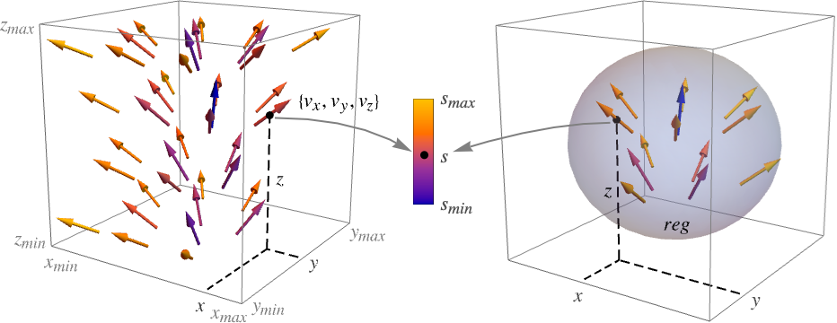
VectorPlot3D[…,{x,y,z}∈reg]
変数{x,y,z}が,幾何学領域 reg にあるものと解釈する.
詳細とオプション
- VectorPlot3Dは,場のプロット,Quiver(震え)プロット,方向プロットとしても知られている.
- VectorPlot3Dは,固定長に正規化された矢印を描いてベクトル場を表示する.デフォルトで,矢印は強度
 によって彩色される.
 - 以下のプロットは集合
 を可視化する.
 - VectorPlot3Dはデフォルトで,3D位置の指定の格子上でベクトル場のベクトルを示す.
- VectorPlot3Dは vi等が評価しても実数にならない場合,対応する矢印を省略する.
- 領域 reg は3Dの任意のRegionQオブジェクトでよい.
- VectorPlot3Dは,事実上Blockを使って変数 x,y および z を局所的なものとして扱う.
- VectorPlot3Dは属性HoldAllを持ち,x,y および z に特定の数値を割り当てた後,はじめて vi等を評価する.場合によっては,Evaluateを使ってまず記号的に vi等を評価した方が効率的かもしれない.
- VectorPlot3DにはGraphics3Dと同じオプションに以下の追加・変更を加えたものが使える. [全オプションのリスト]
-
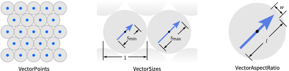
BoxRatios {1,1,1} 縦横比 ClippingStyle Automatic ベクトル範囲の外側の矢印の表示方法 EvaluationMonitor None すべての関数評価で評価される式 Method Automatic プロットに使用するメソッド PerformanceGoal $PerformanceGoal パフォーマンスのどの面について最適化するか PlotLegends None 含める凡例 PlotRange {Full,Full,Full} 含める x, y, z 値の範囲 PlotRangePadding Automatic 値の範囲をどの程度充填するか PlotTheme $PlotTheme プロットの全体的なテーマ RegionBoundaryStyle Automatic プロットの領域の境界スタイルをどうするか RegionFunction (True&) どの領域を含めるかを決める ScalingFunctions None 個々の座標のスケール方法 VectorAspectRatio Automatic 矢印の縦横比 VectorColorFunction Automatic ベクトルの彩色方法 VectorColorFunctionScaling True VectorColorFunctionの引数をスケールするかどう VectorMarkers Automatic 矢印に使う形状 VectorPoints Automatic プロットするベクトルの数または置き方 VectorRange Automatic 表示するベクトルの長さの範囲 VectorScaling None 矢印サイズをどのようにスケールするか VectorSizes Automatic 表示された矢印のサイズ VectorStyle Automatic ベクトルの描き方 WorkingPrecision MachinePrecision 内部計算に使う精度 - 個々の矢印は,各点の周りの境界円内におさまるようにスケールされる.
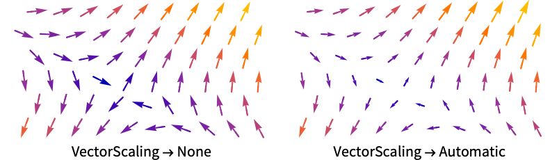
- VectorScalingは,VectorSizesで与えられる sminから smaxの矢印のサイズの範囲にベクトルの大きさをスケールする.
- VectorScalingAutomaticは,ベクトルの大きさによって矢印の長さをスケールする.
- 次は,よく使われるマーカーである.
-
"Arrow3D" 3Dの矢印の形をしたマーカー 
"Arrow" 2Dの矢印の形をしたマーカー 
"Tube" 場の方向に沿ったチューブ片のマーカー 
"Segment" 場の方向に沿った線分 - VectorColorFunctionNoneは,VectorStyleで指定されたスタイルで矢印を描く.
- RegionFunctionおよびVectorColorFunction内の関数に渡される引数は x,y,z,vx,vy,vz,Norm[{vx,vy,vz}]である.
- 次は,ScalingFunctionsの可能な設定である.
-
{sx,sy,sz} x,y,z の各軸をスケールする - 次は,よく使われる組込みのスケーリング関数 s である.
-
"Log" 
自動的に目盛ラベルを付ける対数スケール "Log10" 
10のベキ乗に目盛を置く,10を底とした対数スケール "SignedLog" 
0と負の数を含む対数に似たスケール "Reverse" 
座標の向きを逆にする "Infinite" 
無限スケール
全オプションのリスト
例題
すべて開く すべて閉じる例 (4)
VectorPlot3D[{x, y, z}, {x, -1, 1}, {y, -1, 1}, {z, -1, 1}]VectorPlot3D[{x, y, z}, {x, -1, 1}, {y, -1, 1}, {z, -1, 1}, PlotLegends -> Automatic]VectorPlot3D[{x, y, z}, {x, -1, 1}, {y, -1, 1}, {z, -1, 1}, VectorMarkers -> "Tube"]VectorPlot3D[{x, y, z}, {x, y, z}∈Ball[]]スコープ (14)
サンプリング (5)
Evaluateを使って,数値割当ての前にベクトル場を記号的に評価する:
VectorPlot3D[Evaluate[D[Sin[x y z], {{x, y, z}}]], {x, -1, 1}, {y, -1, 1}, {z, -1, 1}, PlotRange -> All, VectorPoints -> 5]VectorPlot3D[{x, y, z}, {x, -1, 1}, {y, -1, 1}, {z, -1, 1}, RegionFunction -> ((#1 #2 #3 > 0)&)]{VectorPlot3D[{x, y, z}, {x, -1, 1}, {y, -1, 1}, {z, -1, 1}, VectorPoints -> Coarse], VectorPlot3D[{x, y, z}, {x, -1, 1}, {y, -1, 1}, {z, -1, 1}, VectorPoints -> Fine]}points = RandomReal[{-1, 1}, {500, 3}];VectorPlot3D[{x, y, z}, {x, -1, 1}, {y, -1, 1}, {z, -1, 1}, VectorPoints -> points]複数のベクトル場をそれぞれの場に異なる色を使ってプロットする:
VectorPlot3D[{{y, -x, z}, {x, y, z}}, {x, -1, 1}, {y, -1, 1}, {z, -1, 1}, VectorColorFunction -> None, VectorPoints -> 5]プレゼンテーション (9)
大きさに従ってスケールされた矢印でベクトル場をプロットする:
VectorPlot3D[{y, -x, z ^ 2}, {x, -1, 1}, {y, -1, 1}, {z, -1, 1}, VectorScaling -> Automatic]VectorPlot3D[{y, -x, z ^ 2}, {x, -1, 1}, {y, -1, 1}, {z, -1, 1}, VectorColorFunction -> None]VectorPlot3D[{y, -x, z}, {x, -1, 1}, {y, -1, 1}, {z, -1, 1}, PlotRange -> All, VectorPoints -> 5, VectorStyle -> "Arrow3D", VectorColorFunction -> "Rainbow"]points = RandomReal[{-1, 1}, {500, 3}];VectorPlot3D[{x, y, z}, {x, -1, 1}, {y, -1, 1}, {z, -1, 1}, VectorScaling -> Automatic, VectorPoints -> points, PlotRange -> All, VectorColorFunction -> Hue]Table[VectorPlot3D[{x, y, z}, {x, -1, 1}, {y, -1, 1}, {z, -1, 1}, VectorPoints -> 5, VectorSizes -> s, PlotLabel -> s], {s, {Small, Large, 2}}]Table[VectorPlot3D[{x, y, z}, {x, -1, 1}, {y, -1, 1}, {z, -1, 1}, VectorPoints -> 5, VectorScaling -> Automatic, VectorSizes -> s, PlotLabel -> s], {s, {Small, Large, 2}}]points = Normalize /@ RandomReal[{-1, 1}, {250, 3}];VectorPlot3D[{{x, y, z}, {z, -y, x + y}}, {x, -1, 1}, {y, -1, 1}, {z, -1, 1}, VectorColorFunction -> None, VectorPoints -> points, PlotLegends -> {"one", "two"}]VectorPlot3D[{x, y, z}, {x, -1, 1}, {y, -1, 1}, {z, -1, 1}, PlotTheme -> "Marketing"]VectorPlot3D[{x, y, z}, {x, 1, 100}, {y, 1, 10}, {z, 1, 10}, ScalingFunctions -> {"Log", None, None}]VectorPlot3D[{x, y, z}, {x, 1, 100}, {y, 1, 100}, {z, 1, 100}, ScalingFunctions -> {None, None, "Reverse"}]オプション (94)
Axes (3)
デフォルトで,Axesが描かれる:
VectorPlot3D[{z, -y, x + y}, {x, -1, 1}, {y, -1, 1}, {z, -1, 1}]VectorPlot3D[{z, -y, x + y}, {x, -1, 1}, {y, -1, 1}, {z, -1, 1}, Axes -> False]{VectorPlot3D[{z, -y, x + y}, {x, -1, 1}, {y, -1, 1}, {z, -1, 1}, Axes -> {True, False, False}], VectorPlot3D[{z, -y, x + y}, {x, -1, 1}, {y, -1, 1}, {z, -1, 1}, Axes -> {False, True, False}], VectorPlot3D[{z, -y, x + y}, {x, -1, 1}, {y, -1, 1}, {z, -1, 1}, Axes -> {False, False, True}]}AxesLabel (4)
VectorPlot3D[{z, -y, x + y}, {x, -1, 1}, {y, -1, 1}, {z, -1, 1}]
VectorPlot3D[{z, -y, x + y}, {x, -1, 1}, {y, -1, 1}, {z, -1, 1}, AxesLabel -> z]VectorPlot3D[{z, -y, x + y}, {x, -1, 1}, {y, -1, 1}, {z, -1, 1}, AxesLabel -> {x, y, z}]VectorPlot3Dで指定された変数に基づくラベルを使う:
VectorPlot3D[{z, -y, x + y}, {x, -1, 1}, {y, -1, 1}, {z, -1, 1}, AxesLabel -> Automatic]AxesOrigin (2)
AxesStyle (4)
VectorPlot3D[{z, -y, x + y}, {x, -1, 1}, {y, -1, 1}, {z, -1, 1}, AxesStyle -> StandardRed]VectorPlot3D[{z, -y, x + y}, {x, -1, 1}, {y, -1, 1}, {z, -1, 1}, AxesStyle -> {{Thick, StandardBrown}, {Thick, StandardBlue}, {Thick, StandardGreen}}]VectorPlot3D[{z, -y, x + y}, {x, -1, 1}, {y, -1, 1}, {z, -1, 1}, AxesStyle -> StandardGreen, TicksStyle -> StandardGray]VectorPlot3D[{z, -y, x + y}, {x, -1, 1}, {y, -1, 1}, {z, -1, 1}, AxesStyle -> StandardGreen, LabelStyle -> StandardGray]BoxRatios (2)
EvaluationMonitor (2)
ListPointPlot3D[Reap[VectorPlot3D[{x, y, z}, {x, -1, 1}, {y, -1, 1}, {z, -1, 1}, EvaluationMonitor :> Sow[{x, y, z}]]][[-1, 1]]]Block[{k = 0}, VectorPlot3D[{x, y, z}, {x, -1, 1}, {y, -1, 1}, {z, -1, 1}, EvaluationMonitor :> k++];k]ImageSize (7)
Tiny,Small,Medium,Largeのような名前付きのサイズを使う:
{VectorPlot3D[{z, -y, x + y}, {x, -1, 1}, {y, -1, 1}, {z, -1, 1}, ImageSize -> Tiny], VectorPlot3D[{z, -y, x + y}, {x, -1, 1}, {y, -1, 1}, {z, -1, 1}, ImageSize -> Small]}{VectorPlot3D[{z, -y, x + y}, {x, -1, 1}, {y, -1, 1}, {z, -1, 1}, ImageSize -> 150], VectorPlot3D[{z, -y, x + y}, {x, -1, 1}, {y, -1, 1}, {z, -1, 1}, AspectRatio -> 1.5, ImageSize -> 150]}{VectorPlot3D[{z, -y, x + y}, {x, -1, 1}, {y, -1, 1}, {z, -1, 1}, ImageSize -> {Automatic, 150}], VectorPlot3D[{z, -y, x + y}, {x, -1, 1}, {y, -1, 1}, {z, -1, 1}, AspectRatio -> 2, ImageSize -> {Automatic, 150}]}{VectorPlot3D[{z, -y, x + y}, {x, -1, 1}, {y, -1, 1}, {z, -1, 1}, ImageSize -> UpTo[200]], VectorPlot3D[{z, -y, x + y}, {x, -1, 1}, {y, -1, 1}, {z, -1, 1}, AspectRatio -> 2, ImageSize -> UpTo[200]]}グラフィックスの幅と高さを指定して,必要な場合はスペースで充填する:
VectorPlot3D[{z, -y, x + y}, {x, -1, 1}, {y, -1, 1}, {z, -1, 1}, ImageSize -> {200, 300}, Background -> StandardBlue]AspectRatioFullと設定すると,使用可能なスペースが塗り潰される:
VectorPlot3D[{z, -y, x + y}, {x, -1, 1}, {y, -1, 1}, {z, -1, 1}, AspectRatio -> Full, ImageSize -> {200, 300}, Background -> StandardBlue]{VectorPlot3D[{z, -y, x + y}, {x, -1, 1}, {y, -1, 1}, {z, -1, 1}, ImageSize -> {UpTo[150], UpTo[100]}], VectorPlot3D[{z, -y, x + y}, {x, -1, 1}, {y, -1, 1}, {z, -1, 1}, AspectRatio -> 2, ImageSize -> {UpTo[150], UpTo[100]}]}ImageSizeFullを使ってオブジェクト内の使用可能なスペースを塗り潰す:
Framed[Pane[VectorPlot3D[{z, -y, x + y}, {x, -1, 1}, {y, -1, 1}, {z, -1, 1}, ImageSize -> Full, Background -> StandardBlue], {200, 200}]]Framed[Pane[VectorPlot3D[{z, -y, x + y}, {x, -1, 1}, {y, -1, 1}, {z, -1, 1}, AspectRatio -> Full, ImageSize -> {Scaled[0.5], Scaled[0.5]}, Background -> StandardBlue], {200, 200}]]PerformanceGoal (2)
PlotLegends (5)
VectorPlot3D[{z, -y, x + y}, {x, -1, 1}, {y, -1, 1}, {z, -1, 1}]VectorPlot3D[{z, -y, x + y}, {x, -1, 1}, {y, -1, 1}, {z, -1, 1}, PlotLegends -> Automatic]VectorPlot3D[{{x, y, z}, {z, -y, x + y}}, {x, -1, 1}, {y, -1, 1}, {z, -1, 1}, PlotLegends -> {"one", "two"}, VectorColorFunction -> None]VectorPlot3D[{{x, y, z}, {z, -y, x + y}}, {x, -1, 1}, {y, -1, 1}, {z, -1, 1}, VectorColorFunction -> None, PlotLegends -> "Expressions"]VectorPlot3D[{{x, y, z}, {z, -y, x + y}}, {x, -1, 1}, {y, -1, 1}, {z, -1, 1}, PlotLegends -> Placed[{"one", "two"}, Below],
VectorColorFunction -> None]PlotRange (9)
VectorPlot3D[{x, y, z}, {x, -1, 1}, {y, -1, 1}, {z, -1, 1}, PlotRange -> Full]VectorPlot3D[{x, y, z}, {x, -1, 1}, {y, -1, 1}, {z, -1, 1}, PlotRange -> All]


VectorPlot3D[{x, y, z}, {x, -1, 1}, {y, -1, 1}, {z, -1, 1}, PlotRange -> 2]
VectorPlot3D[{x, y, z}, {x, -1, 1}, {y, -1, 1}, {z, -1, 1}, PlotRange -> {{-1, 2}, Automatic, Automatic}]
VectorPlot3D[{x, y, z}, {x, -1, 1}, {y, -1, 1}, {z, -1, 1}, PlotRange -> {{0, Full}, Automatic, Automatic}]
VectorPlot3D[{x, y, z}, {x, -1, 1}, {y, -1, 1}, {z, -1, 1}, PlotRange -> {Full, {0, 2}, Automatic}]
VectorPlot3D[{x, y, z}, {x, -1, 1}, {y, -1, 1}, {z, -1, 1}, PlotRange -> {Full, {Full, 3}, Automatic}]
VectorPlot3D[{x, y, z}, {x, -1, 1}, {y, -1, 1}, {z, -1, 1}, PlotRange -> {Full, Full, {-2, 2}}]


VectorPlot3D[{x, y, z}, {x, -1, 1}, {y, -1, 1}, {z, -1, 1}, PlotRange -> {{-2, 1.5}, {-1, 2}, {0, 1}}]PlotRangePadding (8)
VectorPlot3D[{x, y, z}, {x, -1, 1}, {y, -1, 1}, {z, -1, 1}, PlotRangePadding -> Automatic]


VectorPlot3D[{x, y, z}, {x, -1, 1}, {y, -1, 1}, {z, -1, 1}, PlotRangePadding -> None]


VectorPlot3D[{x, y, z}, {x, -1, 1}, {y, -1, 1}, {z, -1, 1}, PlotRangePadding -> 1]


VectorPlot3D[{x, y, z}, {x, -1, 1}, {y, -1, 1}, {z, -1, 1}, PlotRangePadding -> Scaled[0.1]]

VectorPlot3D[{x, y, z}, {x, -1, 1}, {y, -1, 1}, {z, -1, 1}, PlotRangePadding -> {1, 0.5}]


VectorPlot3D[{x, y, z}, {x, -1, 1}, {y, -1, 1}, {z, -1, 1}, PlotRangePadding -> {1, 0.5, 2}]
VectorPlot3D[{x, y, z}, {x, -1, 1}, {y, -1, 1}, {z, -1, 1}, PlotRangePadding -> {Automatic, Automatic, 2}]VectorPlot3D[{x, y, z}, {x, -1, 1}, {y, -1, 1}, {z, -1, 1}, PlotRangePadding -> {Automatic, Scaled[0.05], 2}]PlotTheme (2)
RegionBoundaryStyle (5)
VectorPlot3D[{x, y, z}, {x, -1, 1}, {y, -1, 1}, {z, -1, 1}, RegionFunction -> Function[{x, y, z}, Abs[x] + Abs[y] < 1]]Noneを使って境界を表示しないようにする:
VectorPlot3D[{x, y, z}, {x, -1, 1}, {y, -1, 1}, {z, -1, 1}, RegionFunction -> Function[{x, y, z}, Abs[x] + Abs[y] < 1], RegionBoundaryStyle -> None]VectorPlot3D[{x, y, z}, {x, -1, 1}, {y, -1, 1}, {z, -1, 1}, RegionFunction -> Function[{x, y, z}, Abs[x] + Abs[y] < 1], RegionBoundaryStyle -> Yellow]VectorPlot3D[{x, y, z}, {x, -1, 1}, {y, -1, 1}, {z, -1, 1}]VectorPlot3D[{x, y, z}, {x, -1, 1}, {y, -1, 1}, {z, -1, 1}, RegionBoundaryStyle -> Yellow]RegionFunction (3)
VectorPlot3D[{x, y, z}, {x, -1, 1}, {y, -1, 1}, {z, -1, 1}, RegionFunction -> ((#1 #2 #3 > 0)&)]場の強度が指定の閾値を超える範囲のみでベクトルをプロットする:
VectorPlot3D[{x, y, z}, {x, -1, 1}, {y, -1, 1}, {z, -1, 1}, RegionFunction -> ((#7 > 1.4)&), VectorPoints -> 10]VectorPlot3D[{x, y, z}, {x, -1, 1}, {y, -1, 1}, {z, -1, 1}, RegionFunction -> ((0.3 < #7 < 0.5 || 1.5 < #7 < 2)&), VectorPoints -> 10]ScalingFunctions (1)
VectorPlot3D[{x, y, z}, {x, 1, 100}, {y, 1, 10}, {z, 1, 10}, ScalingFunctions -> {"Log", None, None}]VectorPlot3D[{x, y, z}, {x, 1, 100}, {y, 1, 100}, {z, 1, 100}, ScalingFunctions -> {None, None, "Reverse"}]Ticks (6)
VectorPlot3D[{x, y, z}, {x, -2, 2}, {y, -2, 2}, {z, -2, 2}]VectorPlot3D[{x, y, z}, {x, -2, 2}, {y, -2, 2}, {z, -2, 2}, Ticks -> None]VectorPlot3D[{x, y, z}, {x, -2, 2}, {y, -2, 2}, {z, -2, 2}, Ticks -> {{-1.5, 0, 1.5}, {-1.5, 0, 1.5}, {-1.5, 0, 1.5}}]VectorPlot3D[{x, y, z}, {x, -2, 2}, {y, -2, 2}, {z, -2, 2}, Ticks -> {{{-1.5, -a}, {0, 0}, {1.5, a}}, {{-1.5, -a}, {0, 0}, {1.5, a}}, {{-1.5, -a}, {0, 0}, {1.5, a}}}]VectorPlot3D[{x, y, z}, {x, -2, 2}, {y, -2, 2}, {z, -2, 2}, Ticks -> {{{-1.5, -a, .1}, {0, 0, .1}, {1.5, a, .1}}, {{-1.5, -a, .05}, {0, 0, .05}, {1.5, a, .05}}, {{-1.5, -a, .15}, {0, 0, .15}, {1.5, a, .15}}}]VectorPlot3D[{x, y, z}, {x, -2, 2}, {y, -2, 2}, {z, -2, 2}, Ticks -> {{{-1.5, -a, .1, Directive[Red, Dashed, Thick]}, {0, 0, .1, Directive[Red, Dashed]}, {1.5, a, .1, Directive[Red]}}, {{-1.5, -a, .05, Directive[Blue, Dashed, Thick]}, {0, 0, .05, Directive[Blue, Dashed]}, {1.5, a, .05, Directive[Blue]}}, {{-1.5, -a, .15, Directive[Darker@Green, Dashed, Thick]}, {0, 0, .15, Directive[Darker@Green, Dashed]}, {1.5, a, .15, Directive[Darker@Green]}}}]TicksStyle (3)
デフォルトで,目盛と目盛ラベルには軸と同じスタイルが使われる:
VectorPlot3D[{x, y, z}, {x, -2, 2}, {y, -2, 2}, {z, -2, 2}, AxesStyle -> StandardRed]VectorPlot3D[{x, y, z}, {x, -2, 2}, {y, -2, 2}, {z, -2, 2}, TicksStyle -> Directive[Bold, StandardRed]]VectorPlot3D[{x, y, z}, {x, -2, 2}, {y, -2, 2}, {z, -2, 2}, TicksStyle -> {Directive[StandardGray, Bold], Directive[Bold, StandardRed], Directive[Bold, StandardBlue]}]VectorAspectRatio (2)
VectorPlot3D[{z y - z x(1 - x^2 - y^2)^2, -z x - z y(1 - x^2 - y^2)^2, z}, {x, -3, 3}, {y, -3, 3}, {z, -3, 3}, VectorAspectRatio -> 0.3]VectorPlot3D[{z y - z x(1 - x^2 - y^2)^2, -z x - z y(1 - x^2 - y^2)^2, z}, {x, -3, 3}, {y, -3, 3}, {z, -3, 3}, VectorAspectRatio -> 0.2]VectorColorFunction (4)
VectorPlot3D[{x, y, z}, {x, -1, 1}, {y, -1, 1}, {z, -1, 1}, VectorColorFunction -> Hue]ColorDataから任意の名前付き色階調度を使う:
VectorPlot3D[{x, y, z}, {x, -1, 1}, {y, -1, 1}, {z, -1, 1}, VectorColorFunction -> "Rainbow"]
VectorPlot3D[{x, y, z}, {x, -1, 1}, {y, -1, 1}, {z, -1, 1}, VectorColorFunction -> Function[{x, y, z, vx, vy, vz, n}, ColorData["ThermometerColors"][x]]]VectorColorFunctionScalingFalseを使ってスケールされていない値を得る:
VectorPlot3D[{x, y, z}, {x, -1, 1}, {y, -1, 1}, {z, -1, 1}, VectorColorFunction -> (ColorData[22][Round[#7]]&), VectorColorFunctionScaling -> False]VectorColorFunctionScaling (4)
VectorPlot3D[{x, y, z}, {x, -1, 1}, {y, -1, 1}, {z, -1, 1}, VectorColorFunction -> Hue]VectorColorFunctionScaling->Falseを使ってスケールされていない値を得る:
VectorPlot3D[{x, y, z}, {x, -1, 1}, {y, -1, 1}, {z, -1, 1}, VectorColorFunction -> (ColorData[22][Round[#7]]&), VectorColorFunctionScaling -> False] 方向にはスケールされていない座標を,
 方向にはスケールされた座標を使う:
VectorPlot3D[{x, y, z}, {x, -1, 1}, {y, -1, 1}, {z, -1, 1}, VectorColorFunction -> Function[{x, y, z, vx, vy, vz, n}, Hue[x, y, 1]], VectorColorFunctionScaling -> {False, True}]VectorPlot3D[{x, y, z}, {x, -1, 1}, {y, -1, 1}, {z, -1, 1}, VectorColorFunction -> (Hue[#7, #2, 1]&), VectorColorFunctionScaling -> {True, True, True, True, False}]VectorMarkers (3)
VectorPlot3D[{x, y, z}, {x, -1, 1}, {y, -1, 1}, {z, -1, 1}]Table[VectorPlot3D[{x, y, z}, {x, -1, 1}, {y, -1, 1}, {z, -1, 1}, VectorMarkers -> m, PlotLabel -> m], {m, {"Tube", "Segment", "Arrow"}}]Placedを使ってベクトル点と相対的な矢印の置き方を制御する:
pts = Flatten[Table[{x, y, z}, {x, -1, 1}, {y, -1, 1}, {z, -1, 1}], 2];Table[Show[VectorPlot3D[{x, y, z}, {x, -1, 1}, {y, -1, 1}, {z, -1, 1}, VectorMarkers -> Placed["Arrow", pos], VectorPoints -> pts],
ListPointPlot3D[pts]], {pos, {"Start", "End"}}]VectorPoints (7)
VectorPlot3D[{x, y, z}, {x, -1, 1}, {y, -1, 1}, {z, -1, 1}, VectorPoints -> Automatic]Table[VectorPlot3D[{x, y, z}, {x, -1, 1}, {y, -1, 1}, {z, -1, 1}, PlotLabel -> k, VectorPoints -> k], {k, {Fine, Coarse}}] ,
,  ,
,  に同数の矢印を使って場のベクトルの構造格子を作成する:
VectorPlot3D[{x, y, z}, {x, -1, 1}, {y, -1, 1}, {z, -1, 1}, VectorPoints -> 5] ,
,  ,
,  に異なる数の矢印を使って場のベクトルの構造格子を作成する:
VectorPlot3D[{x, y, z}, {x, -1, 1}, {y, -1, 1}, {z, -1, 1}, VectorPoints -> {4, 7, 9}]VectorPlot3D[{x, y, z}, {x, -1, 1}, {y, -1, 1}, {z, -1, 1}, VectorPoints -> RandomReal[{-1, 1}, {300, 3}]]Table[VectorPlot3D[{x, y, z}, {x, -1, 1}, {y, -1, 1}, {z, -1, 1}, PlotLabel -> n, VectorPoints -> n], {n, 4, 10, 3}]points = {{-1, -1, -1}, {-1, 1, 1}, {1, -1, -1}, {1, 1, 1}};Show[VectorPlot3D[{x, y, z}, {x, -2, 2}, {y, -2, 2}, {z, -2, 2}, VectorPoints -> points, PlotRange -> 2], Graphics3D[{Red, Sphere[points, 0.15]}]]Show[VectorPlot3D[{x, y, z}, {x, -2, 2}, {y, -2, 2}, {z, -2, 2}, VectorPoints -> points, PlotRange -> 2, VectorMarkers -> "Start"], Graphics3D[{Red, Sphere[points, 0.15]}]]VectorRange (4)
大きさが非常に小さいまたは非常に大きいベクトルのクリッピングは自動的に行われる:
VectorPlot3D[({x, y, z}/Norm[{x, y, z}]^3), {x, -3, 3}, {y, -3, 3}, {z, -3, 3}, VectorRange -> Automatic]VectorPlot3D[({x, y, z}/Norm[{x, y, z}]^3), {x, -3, 3}, {y, -3, 3}, {z, -3, 3}, VectorRange -> {0.1, 2}]VectorPlot3D[({x, y, z}/Norm[{x, y, z}]^3), {x, -3, 3}, {y, -3, 3}, {z, -3, 3}, VectorRange -> {0.1, 2}, ClippingStyle -> None]VectorPlot3D[({x, y, z}/Norm[{x, y, z}]^3), {x, -3, 3}, {y, -3, 3}, {z, -3, 3}, VectorRange -> All]VectorStyle (2)
VectorColorFunctionは,VectorStyleでは色より優先順位が高い:
VectorPlot3D[{x, y, z}, {x, -1, 1}, {y, -1, 1}, {z, -1, 1}, VectorStyle -> Red]VectorColorFunction→Noneを使ってVectorStyleで色を指定する:
VectorPlot3D[{x, y, z}, {x, -1, 1}, {y, -1, 1}, {z, -1, 1}, VectorStyle -> StandardRed, VectorColorFunction -> None]アプリケーション (1)
位置  における点電荷
  の集合から構築された静電ポテンシャル:
electroStaticPotential[q_, p_, r_] := Sum[ (q[[i]]/Norm[r - p[[i]]]), {i, Length[q]}]electroStaticPotential[{Subscript[q, 1], Subscript[q, 2]}, {{Subscript[x, 1], Subscript[y, 1], Subscript[z, 1]}, {Subscript[x, 2], Subscript[y, 2], Subscript[z, 2]}}, {x, y, z}]//TraditionalForm

electricField[{q1_, q2_}, {{x1_, y1_, z1_}, {x2_, y2_, z2_}}] = -D[electroStaticPotential[{q1, q2}, {{x1, y1, z1}, {x2, y2, z2}}, {x, y, z}], {{x, y, z}}] /. Derivative[1][Abs][x_] :> (x/Sqrt[x^2]);

c = ContourPlot3D[Evaluate[electroStaticPotential[{1, -1}, {{-1, 0, 0}, {1, 0, 0}}, {x, y, z}]], {x, -6, 6}, {y, 0, 4}, {z, -4, 4}, Contours -> {-0.75, -0.25, -0.1, 0, 0.1, 0.25, 0.75}, ContourStyle -> Table[Hue[i / 7, 1, 1, 0.5], {i, 0, 6}], Mesh -> None]

v = VectorPlot3D[electricField[{1, -1}, {{-1, 0, 0}, {1, 0, 0}}], {x, -6, 6}, {y, 0, 4}, {z, -4, 4}, VectorPoints -> 5]Show[v, c]特性と関係 (14)
ListVectorPlot3Dを使ってデータを可視化する:
vectors = Table[{x, y, z}, {x, -1, 1, .1}, {y, -1, 1, .1}, {z, -1, 1, .1}];ListVectorPlot3D[vectors]SliceVectorPlot3Dで曲面に沿ってベクトルをプロットする:
SliceVectorPlot3D[{x, y, z}, {x, -1, 1}, {y, -1, 1}, {z, -1, 1}]ListSliceVectorPlot3Dで曲面上にデータベクトルをプロットする:
data = Table[{z, x, x + y}, {x, -1, 1}, {y, -1, 1}, {z, -1, 1}];ListSliceVectorPlot3D[data, "CenterPlanes"]StreamPlot3Dを使って3Dベクトル場の流線をプロットする:
StreamPlot3D[{z, -x, y}, {x, -2, 2}, {y, -2, 2}, {z, -2, 2}]ListStreamPlot3Dを使ってデータでプロットする:
data = Table[{z, -x, y}, {x, -2, 2}, {y, -2, 2}, {z, -2, 2}];ListStreamPlot3D[data]VectorDisplacementPlotを使って変位ベクトル場の指定の領域における影響を可視化する:
VectorDisplacementPlot[{-1 - x ^ 2 + y, 1 + x - y ^ 2}, {x, y}∈Annulus[], VectorPoints -> Automatic]ListVectorDisplacementPlotを使って領域における変位ベクトル場の影響を可視化する:
data = Table[{{x, y}, {x + y, 1 + x - y}}, {x, -3, 3, 0.2}, {y, -3, 3, 0.2}];ListVectorDisplacementPlot[data, Polygon[{{3, 3}, {0, 1}, {-3, 3}, {-3, -3}, {0, -1}, {3, -3}}], VectorPoints -> Automatic]VectorDisplacementPlot3Dを使って変位ベクトル場の指定された3D領域における影響を可視化する:
VectorDisplacementPlot3D[{-y, x, x + z}, {x, -2, 2}, {y, -2, 2}, {z, -2, 2}, VectorPoints -> "Boundary"]ListVectorDisplacementPlot3Dを使って指定された領域における3D変位ベクトル場データの影響を可視化する:
data = Table[{{x, y, z}, {-y, x, x + z}}, {x, -2, 2}, {y, -2, 2}, {z, -2, 2}];ListVectorDisplacementPlot3D[data, VectorPoints -> "Boundary"]VectorPlotを2Dベクトルのプロットに使う:
VectorPlot[{y, -x}, {x, -2, 2}, {y, -2, 2}]ListVectorPlotを使ってデータでプロットする:
data = Table[{y, -x}, {x, -2, 2}, {y, -2, 2}];ListVectorPlot[data]StreamPlotを使ってベクトルの代りに流線でプロットする:
StreamPlot[{-1 - x ^ 2 + y, 1 + x - y ^ 2}, {x, -3, 3}, {y, -3, 3}]data = Table[{-1 - x ^ 2 + y, 1 + x - y ^ 2}, {x, -3, 3, 0.1}, {y, -3, 3, 0.1}];ListStreamPlot[data]VectorDensityPlotを使ってスカラー場の密度プロットを加える:
VectorDensityPlot[{-1 - x ^ 2 + y, 1 + x - y ^ 2}, {x, -3, 3}, {y, -3, 3}]StreamDensityPlotを使ってベクトルの代りに流線をプロットする:
StreamDensityPlot[{-1 - x ^ 2 + y, 1 + x - y ^ 2}, {x, -3, 3}, {y, -3, 3}]ListVectorDensityPlotまたはListStreamDensityPlotをデータのプロットに使う:
data = Table[{{x, y} = RandomReal[{-1.5, 1.5}, {2}], {{y, x - x ^ 3}, Abs[x + y]}}, {300}];{ListVectorDensityPlot[data], ListStreamDensityPlot[data]}LineIntegralConvolutionPlotを使ってベクトル場の線積分たたみ込みをプロットする:
LineIntegralConvolutionPlot[{-1 - x ^ 2 + y, 1 + x - y ^ 2}, {x, -3, 3}, {y, -3, 3}]ComplexVectorPlot[z + 1 / z, {z, 2}]ComplexStreamPlotでベクトルではなく流れをプロットする:
ComplexStreamPlot[z^2 + 1, {z, 2}]GeoVectorPlotを使って地球の上にベクトルプロットを生成する:
coords = Flatten[Table[{lat, long}, {long, -180, 180, 30}, {lat, -75, 75, 15}], 1];vects = Table[{RandomReal[], Quantity[RandomReal[{0, 360}], "AngularDegrees"]}, {Length[coords]}];GeoVectorPlot[GeoVector[GeoPosition[coords] -> vects]]GeoStreamPlotを使ってベクトルの代りに流れを使う:
GeoStreamPlot[GeoVector[GeoPosition[coords] -> vects]]テキスト
Wolfram Research (2008), VectorPlot3D, Wolfram言語関数, https://reference.wolfram.com/language/ref/VectorPlot3D.html (2022年に更新).
CMS
Wolfram Language. 2008. "VectorPlot3D." Wolfram Language & System Documentation Center. Wolfram Research. Last Modified 2022. https://reference.wolfram.com/language/ref/VectorPlot3D.html.
APA
Wolfram Language. (2008). VectorPlot3D. Wolfram Language & System Documentation Center. Retrieved from https://reference.wolfram.com/language/ref/VectorPlot3D.html