


ComplexRegionPlot
ComplexRegionPlot[pred,{z,zmin,zmax}]
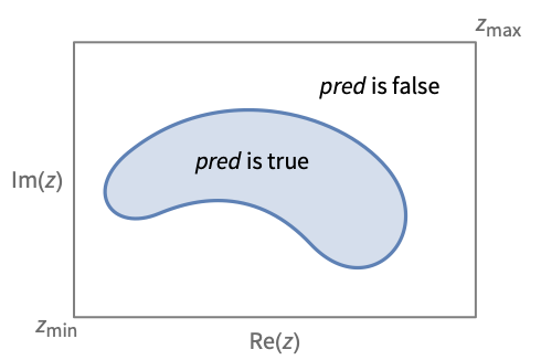
makes a plot showing the region in the complex plane for which pred is True.
ComplexRegionPlot[{pred1,pred2,…},{z,zmin,zmax}]
plots regions given by the multiple predicates predi.
Details and Options
- The predicate predi can be any logical combination of inequalities. The predi will typically involve functions like Re, Im, Abs and Arg that extract real components from complex numbers for comparison purposes.
- The region plotted by ComplexRegionPlot can contain disconnected parts.
- ComplexRegionPlot[pred,{z,n}] is equivalent to ComplexRegionPlot[pred,{z,-n-n I,n+n I}].
- ComplexRegionPlot treats the variable z as local, effectively using Block.
- ComplexRegionPlot has attribute HoldAll and evaluates pred only after assigning specific numerical values to z. In some cases, it may be more efficient to use Evaluate to evaluate pred symbolically first.
- The following wrappers w can be used for the predi:
-
Annotation[predi,label] provide an annotation for the predi Button[predi,action] evaluate action when the curve for predi is clicked Callout[predi,label] label the region with a callout Callout[predi,label,pos] place the callout at relative position pos EventHandler[predi,events] define a general event handler for predi Hyperlink[predi,uri] make the region a hyperlink Labeled[predi,label] label the region Labeled[predi,label,pos] place the label at relative position pos Legended[predi,label] identify the region in a legend PopupWindow[predi,cont] attach a popup window to the region StatusArea[predi,label] display in the status area on mouseover Style[predi,styles] show the region using the specified styles Tooltip[predi,label] attach a tooltip to the region Tooltip[predi] use regions as tooltips - Wrappers w can be applied at multiple levels:
-
w[predi] wrap the predi w[{predi,…}] wrap a collection of predi w1[w2[…]] use nested wrappers - Callout, Labeled and Placed can use the following positions pos:
-
Automatic automatically placed labels Above, Below, Before, After positions around the region z position near z {pos,epos} epos in label placed at relative position pos of the region - ComplexRegionPlot has the same options as Graphics, with the following additions and changes: [List of all options]
-
AspectRatio 1 ratio of height to width BoundaryStyle Automatic the style for the boundary of each region ColorFunction Automatic how to color the interior of each region ColorFunctionScaling True whether to scale the argument to ColorFunction EvaluationMonitor None expression to evaluate at every function evaluation Frame True whether to draw a frame around the plot LabelingSize Automatic maximum size of callouts and labels MaxRecursion Automatic the maximum number of recursive subdivisions allowed Mesh None how many mesh lines to draw MeshFunctions {#1&,#2&} what mesh lines to draw MeshShading None how to shade regions between mesh lines MeshStyle Automatic the style for mesh lines Method Automatic the method to use for refining regions PerformanceGoal $PerformanceGoal aspects of performance to try to optimize PlotLabels None labels to use for curves PlotLegends None legends for regions PlotPoints Automatic initial number of sample points PlotRange Full the range of values to include in the plot PlotRangeClipping True whether to clip at the plot range PlotRangePadding Automatic how much to pad the range of values PlotStyle Automatic graphics directives to specify the style for regions PlotTheme $PlotTheme overall theme for the plot TextureCoordinateFunction Automatic how to determine texture coordinates TextureCoordinateScaling True whether to scale arguments to TextureCoordinateFunction WorkingPrecision MachinePrecision the precision used in internal computations - Typical settings for PlotLegends include:
-
None no legend Automatic automatically determine the legend "Expressions" use f1, f2, … as the legend labels {lbl1,lbl2,…} use lbl1, lbl2, … as the legend labels Placed[lspec,…] specify placement for the legend - PlotStylesty specifies the styles to use for each curve. Possible settings include:
-
{sty1,sty2,…} sequence of styles for the datasets <"key"val,…> styling elements for different levels of data - The accepted keys are:
-
"Base" overall style for all the fi "Functions" list of styles styi for each fi - ColorData["DefaultPlotColors"] gives the default sequence of colors used by PlotStyle.
- ComplexRegionPlot initially evaluates pred at a grid of equally spaced sample points specified by PlotPoints. Then it uses an adaptive algorithm to subdivide at most MaxRecursion times, attempting to find the boundaries of all regions in which pred is True.
- You should realize that since it uses only a finite number of sample points, it is possible for ComplexRegionPlot to miss regions in which pred is True. To check your results, you should try increasing the settings for PlotPoints and MaxRecursion.
- With the default setting PlotRange->Full, ComplexRegionPlot will explicitly include the full ranges zmin to zmax for z.
- ComplexRegionPlot can in general only find regions of positive measure; it cannot find regions that are just lines or points.
- The argument supplied to functions in MeshFunctions is z. ColorFunction and TextureCoordinateFunction are by default supplied with scaled versions of of Re[z], Im[z], Abs[z], Arg[z].
List of all options
Examples
open all close allBasic Examples (5)
Plot a region in the complex plane defined by an inequality:
ComplexRegionPlot[Abs[z] ≤ 1, {z, -1 - I, 1 + I}]Specifying the domain with {z,1} is equivalent to {z,-1-,1+}:
ComplexRegionPlot[Abs[z] ≤ 1, {z, 1}]Plot a region defined by logical combinations of inequalities:
ComplexRegionPlot[0 < Arg[z] < 2π / 3, {z, 5}]ComplexRegionPlot[{Re[z ^ 2] < 1, Im[z ^ 2] < 1}, {z, 2}]ComplexRegionPlot[Abs[z] ≤ 1 && Abs[Arg[z]] > π / 4, {z, -1 - I, 1 + I}, PlotStyle -> Yellow]Scope (23)
Sampling (3)
More points are sampled near the boundary of the region:
ComplexRegionPlot[Abs[Nest[(# ^ 2 + z)&, z, 8]] < 2, {z, -2 - 1.5I, 1 + 1.5I}, Mesh -> All]Use PlotPoints and MaxRecursion to control adaptive sampling:
Table[ComplexRegionPlot[1 < Abs[Sin[2 z] Cosh[2 z]] < 4, {z, -2 - 2I, 2 + 2I}, PlotPoints -> pp, MaxRecursion -> mr, Mesh -> None], {mr, {0, 2}}, {pp, {5, 15}}]Use logical combinations of regions:
ComplexRegionPlot[Re[z^2] ≤ 2 && Im[z^2] > 1, {z, -3 - 3I, 3 + 3I}]Labeling and Legending (9)
Label regions with Labeled:
ComplexRegionPlot[Labeled[Abs[z] < 1, "disk", Above], {z, -1.5 - 1.5I, 1.5 + 1.5I}]ComplexRegionPlot[{Labeled[Abs[z] < 1, "disk", Right], Labeled[Re[z] < 1, "rectangle", Below]}, {z, -1.5 - 1.5I, 1.5 + 1.5I}]Place the labels in different positions:
Table[ComplexRegionPlot[Labeled[Abs[z] < 1, "disk", pos], {z, -1.5 - 1.5I, 1.5 + 1.5I}, PlotLabel -> pos], {pos, {Top, Bottom, Left, Right}}]Label regions with Callout:
ComplexRegionPlot[Callout[1 < Abs[Sin[2 z] Sinh[2 z]] < 6, "region", {1, 1}], {z, -2 - 2I, 2 + 2I}]ComplexRegionPlot[{Callout[1 < Abs[Sin[2 z] Sinh[2 z]] < 6, "region", {1, 1}], Callout[Abs[z] < 2, "disk", {1, -1}]}, {z, -2 - 2I, 2 + 2I}]Callout leader is turned off when label is inside the region:
ComplexRegionPlot[Callout[Abs[Sin[2 z] Sinh[2 z]] < 6, "region", {0, 0}], {z, -2 - 2I, 2 + 2I}]Add a legend with PlotLegends:
ComplexRegionPlot[{1 < Abs[Sin[2 z] Sinh[2 z]] < 6, Abs[z] < 2}, {z, -2 - 2I, 2 + 2I}, PlotLegends -> "Expressions"]Use editable placeholders in the legend:
ComplexRegionPlot[{1 < Abs[Sin[2 z] Sinh[2 z]] < 6, Abs[z] < 2}, {z, -2 - 2I, 2 + 2I}, PlotLegends -> Automatic]Add legends with Legended:
ComplexRegionPlot[{Legended[1 < Abs[Sin[2 z] Sinh[2 z]] < 6, "region"], Legended[Abs[z] < 2, "disk"]}, {z, -2 - 2I, 2 + 2I}]Presentation (11)
Provide an explicit PlotStyle for the region:
ComplexRegionPlot[Abs[z] ≤ 1 && Abs[Arg[z]] > π / 4, {z, -1 - I, 1 + I}, PlotStyle -> Yellow]Provide an explicit BoundaryStyle for the region boundary:
ComplexRegionPlot[Abs[z] ≤ 1 && Abs[Arg[z]] > π / 4, {z, -1 - I, 1 + I}, PlotStyle -> Yellow, BoundaryStyle -> Dashed]Add descriptive labels for the plot, the axes and the regions:
ComplexRegionPlot[{3 ≤ Abs[z] ≤ 4, Abs[z] < 2}, {z, -4 - 4I, 4 + 4I}, FrameLabel -> {"real", "imaginary"}, PlotLabel -> "shapes", PlotLabels -> {"annulus", "disk"}]Use a combination of methods to label regions:
ComplexRegionPlot[{Callout[3 ≤ Abs[z] ≤ 4, "annulus"], Labeled[Abs[z] < 2, "disk", Below]}, {z, -4 - 4I, 4 + 4I}]Use a legend for multiple regions:
ComplexRegionPlot[{3 ≤ Abs[z] ≤ 4, Abs[z] < 2}, {z, -4 - 4I, 4 + 4I}, PlotLegends -> "Expressions"]Produce a legend with editable placeholders:
ComplexRegionPlot[{3 ≤ Abs[z] ≤ 4, Abs[z] < 2}, {z, -4 - 4I, 4 + 4I}, PlotLegends -> Automatic]Use a legend for colored regions:
ComplexRegionPlot[2 ≤ Abs[z] ≤ 4, {z, -4 - 4I, 4 + 4I}, ColorFunction -> Hue, PlotLegends -> Automatic]ComplexRegionPlot[2 ≤ Abs[z] ≤ 4, {z, -4 - 4I, 4 + 4I}, Mesh -> 8, MeshStyle -> Directive[Red, Dashed]]Style the areas between mesh lines:
ComplexRegionPlot[2 ≤ Abs[z] ≤ 4, {z, -4 - 4I, 4 + 4I}, Mesh -> 8, MeshShading -> {{Yellow, Orange}, {Pink, Red}}]Color the region with an overlay density:
ComplexRegionPlot[Abs[Nest[(# ^ 2 + z)&, z, 8]] < 2, {z, -2 - 1.5I, 1 + 1.5I}, ColorFunction -> Function[{re, im, abs, arg}, Hue[Nest[(# ^ 2 + re)&, re, 8]]], ColorFunctionScaling -> False, PlotPoints -> 50]ComplexRegionPlot[2 ≤ Abs[z] ≤ 4, {z, -4 - 4I, 4 + 4I}, PlotTheme -> "Scientific"]Options (59)
BoundaryStyle (4)
ComplexRegionPlot[Abs[z^4 - z / 5 + 1] ≤ 1, {z, -1 - I, 1 + I}]Use None to show regions without any boundary:
ComplexRegionPlot[Abs[z^4 - z / 5 + 1] ≤ 1, {z, -1 - I, 1 + I}, BoundaryStyle -> None]ComplexRegionPlot[Abs[z^4 - z / 5 + 1] ≤ 1, {z, -1 - I, 1 + I}, BoundaryStyle -> Red]Use a thicker dashed boundary:
ComplexRegionPlot[Abs[z^4 - z / 5 + 1] ≤ 1, {z, -1 - I, 1 + I}, BoundaryStyle -> Directive[Thickness[Medium], Dashed]]ColorFunction (5)
Color regions by scaled Re[z], Im[z], Abs[z] or Arg[z]:
{
	ComplexRegionPlot[Abs[z] < 2, {z, -2 - 2I, 2 + 2I}, ColorFunction -> (Hue[#1]&)],
	ComplexRegionPlot[Abs[z] < 2, {z, -2 - 2I, 2 + 2I}, ColorFunction -> (Hue[#2]&)],
	ComplexRegionPlot[Abs[z] < 2, {z, -2 - 2I, 2 + 2I}, ColorFunction -> (Hue[#3]&)],
	ComplexRegionPlot[Abs[z] < 2, {z, -2 - 2I, 2 + 2I}, ColorFunction -> (Hue[#4]&)]
	}
Named color functions use the scaled Arg[z] direction:
ComplexRegionPlot[Abs[z] < 1, {z, -1 - I, 1 + I}, ColorFunction -> "Rainbow"]Color regions according to a function of ![]() :
:
ComplexRegionPlot[Abs[z^4 - z / 5 + 1] ≤ 1, {z, -1 - I, 1 + I}, ColorFunction -> Function[{z}, ColorData["SolarColors"][Abs[z]]], ColorFunctionScaling -> False]ColorFunction has higher priority than PlotStyle:
ComplexRegionPlot[Abs[z^4 - z / 5 + 1] ≤ 1, {z, -1 - I, 1 + I}, ColorFunction -> "DarkRainbow", PlotStyle -> Directive[Opacity[0.5], Red]]ColorFunction has lower priority than MeshShading:
ComplexRegionPlot[Abs[z^4 - z / 5 + 1] ≤ 1, {z, -1 - I, 1 + I}, Mesh -> 30, MeshShading -> {{Gray, Automatic}, {Automatic, Gray}}, ColorFunction -> "DarkRainbow"]ColorFunctionScaling (1)
Use unscaled Re[z], Im[z], Abs[z] or Arg[z] for coloring the regions:
{
	ComplexRegionPlot[Abs[z] < 2, {z, -2 - 2I, 2 + 2I}, ColorFunction -> (Hue[#1]&), ColorFunctionScaling -> False],
	ComplexRegionPlot[Abs[z] < 2, {z, -2 - 2I, 2 + 2I}, ColorFunction -> (Hue[#2]&), ColorFunctionScaling -> False],
	ComplexRegionPlot[Abs[z] < 2, {z, -2 - 2I, 2 + 2I}, ColorFunction -> (Hue[#3]&), ColorFunctionScaling -> False],
	ComplexRegionPlot[Abs[z] < 2, {z, -2 - 2I, 2 + 2I}, ColorFunction -> (Hue[#4]&), ColorFunctionScaling -> False]
	}
LabelingSize (2)
Textual labels are shown at their actual sizes:
ComplexRegionPlot[Callout[Abs[z] ≤ 1 && Abs[Arg[z]] > π / 4, "region"], {z, -1 - I, 1 + I}, PlotStyle -> Yellow]ComplexRegionPlot[Callout[Abs[z] ≤ 1 && Abs[Arg[z]] > π / 4, "region"], {z, -1 - I, 1 + I}, PlotStyle -> Yellow, LabelingSize -> 25]MaxRecursion (1)
Mesh (7)
ComplexRegionPlot[Abs[z] ≤ 1, {z, -1 - I, 1 + I}]Show the initial and final sampling meshes:
{ComplexRegionPlot[Abs[z] ≤ 1, {z, -1 - I, 1 + I}, Mesh -> Full],
	ComplexRegionPlot[Abs[z] ≤ 1, {z, -1 - I, 1 + I}, Mesh -> All]}
Use 10 mesh lines in each direction:
ComplexRegionPlot[Abs[z] ≤ 1, {z, -1 - I, 1 + I}, Mesh -> 10]Use 3 mesh lines in the Re[z] direction and 6 mesh lines in the Im[z] direction:
ComplexRegionPlot[Abs[z] ≤ 1, {z, -1 - I, 1 + I}, Mesh -> {3, 6}]Use mesh lines at specific values:
ComplexRegionPlot[Abs[z] ≤ 1, {z, -1 - I, 1 + I}, Mesh -> {{-1 / 2, 1 / 2}, {0}}]Use different styles for different mesh lines:
ComplexRegionPlot[Abs[z] ≤ 1, {z, -1 - I, 1 + I}, Mesh -> {{{-1 / 2, Red}, {1 / 2, Red}}, {{0, Dashed}}}]Mesh lines apply to the whole region, not each component:
ComplexRegionPlot[Abs[z] > 1 && Pi / 4 < Abs[Arg[z]] < 3Pi / 4, {z, -2 - 2I, 2 + 2I}, Mesh -> 10]MeshFunctions (2)
Mesh lines in the Re[z] and Im[z] directions:
{ComplexRegionPlot[Abs[z] ≤ 1, {z, -1 - I, 1 + I}, Mesh -> 10, MeshFunctions -> {Re[#]&}], ComplexRegionPlot[Abs[z] ≤ 1, {z, -1 - I, 1 + I}, Mesh -> 10, MeshFunctions -> {Im[#]&}]}Mesh lines at fixed radii from the origin:
ComplexRegionPlot[Abs[z] ≤ 1, {z, -1 - I, 1 + I}, Mesh -> 10, MeshFunctions -> {Abs[#]&}]MeshShading (4)
Use None to remove regions:
ComplexRegionPlot[Abs[z] ≤ 1, {z, -1 - I, 1 + I}, Mesh -> 8, MeshFunctions -> {Re[#] - Im[#]&}, MeshShading -> {Red, None}]Lay a checkerboard pattern over a region:
ComplexRegionPlot[Abs[z] ≤ 1, {z, -1 - I, 1 + I}, Mesh -> 10, MeshShading -> {{Red, Yellow}, {Pink, Orange}}]MeshShading has a higher priority than PlotStyle:
ComplexRegionPlot[Abs[z] ≤ 1, {z, -1 - I, 1 + I}, Mesh -> 10, PlotStyle -> Blue, MeshShading -> {{Automatic, Green}, {Green, Automatic}}]MeshShading has a higher priority than ColorFunction:
ComplexRegionPlot[Abs[z] ≤ 1, {z, -1 - I, 1 + I}, Mesh -> 10, PlotStyle -> Blue, MeshShading -> {{Automatic, None}, {None, Automatic}}, ColorFunction -> "DarkRainbow"]MeshStyle (2)
ComplexRegionPlot[Abs[z] ≤ 1, {z, -1 - I, 1 + I}, Mesh -> 5, MeshStyle -> Red]Use red mesh lines in the Re[z] direction and dashed mesh lines in the Im[z] direction:
ComplexRegionPlot[Abs[z] ≤ 1, {z, -1 - I, 1 + I}, Mesh -> 5, MeshStyle -> {Red, Dashed}]PerformanceGoal (2)
Generate a higher-quality plot:
Timing[ComplexRegionPlot[1 < Abs[Sin[2 z] Cosh[2 z]] < 3, {z, -2 - 2I, 2 + 2I}, PerformanceGoal -> "Quality"]]Emphasize performance, possibly at the cost of quality:
Timing[ComplexRegionPlot[1 < Abs[Sin[2 z] Cosh[2 z]] < 3, {z, -2 - 2I, 2 + 2I}, PerformanceGoal -> "Speed"]]PlotLabels (5)
ComplexRegionPlot[1 < Abs[Sin[5 z] Cosh[2z]] < 3, {z, -1 - I, 1 + I}, PlotLabels -> "label"]Place the label above the region:
ComplexRegionPlot[1 < Abs[Sin[5 z] Cosh[2z]] < 3, {z, -1 - I, 1 + I}, PlotLabels -> Placed["island", Above]]Place the label inside the region:
ComplexRegionPlot[1 < Abs[Sin[5 z] Cosh[2z]] < 3, {z, -1 - I, 1 + I}, PlotLabels -> Placed["hole", Center]]Use Callout to place the label:
ComplexRegionPlot[{1 < Abs[Sin[5 z] Cosh[2z]] < 3}, {z, -1 - I, 1 + I}, PlotLabels -> Callout["label", {0.5, 0.5}]]ComplexRegionPlot[{1 < Abs[Sin[5 z] Cosh[2z]] < 3, Abs[z ^ 2 + 1] > 1}, {z, -1 - I, 1 + I}, PlotLabels -> {Callout["label1", Below], Callout["label2", After]}]PlotLegends (8)
ComplexRegionPlot[Abs[Nest[(# ^ 2 + z)&, z, 8]] < 2, {z, -2 - 1.5I, 1 + 1.5I}, PlotLegends -> All]Use legends for multiple regions:
ComplexRegionPlot[{1 < Abs[Sin[5 z] Cosh[2z]] < 3, Abs[z ^ 2 + 1] > 1}, {z, -1 - I, 1 + I}, PlotLegends -> Automatic]Use automatic legends for a gradient colored region:
ComplexRegionPlot[Abs[z] ≤ 1, {z, -1 - I, 1 + I}, ColorFunction -> "GreenPinkTones", PlotLegends -> Automatic]PlotLegends automatically picks up styles:
ComplexRegionPlot[{Abs[z ^ 2 + 1] > 1, 1 < Abs[Sin[5 z] Cosh[2z]] < 3}, {z, -1 - I, 1 + I}, PlotStyle -> {StandardRed, StandardBlue}, PlotLegends -> Automatic]Use functions as legend texts:
ComplexRegionPlot[{1 < Abs[Sin[5 z] Cosh[2z]] < 3, Abs[z ^ 2 + 1] > 1}, {z, -1 - I, 1 + I}, PlotLegends -> "Expressions"]ComplexRegionPlot[{Abs[z - 1] < 1, Abs[z + 1] < 1}, {z, -2 - 2I, 2 + 2I}, PlotLegends -> {"left", "right"}]Use Placed to change legend position:
Table[ComplexRegionPlot[{Abs[z - 1] < 1, Abs[z + 1] < 1}, {z, -2 - 2I, 2 + 2I}, PlotLegends -> Placed[Automatic, pos], PlotLabel -> pos], {pos, {Before, After, Above, Below}}]Use SwatchLegend to change legend appearance:
ComplexRegionPlot[{Abs[z - 1] < 1, Abs[z + 1] < 1}, {z, -2 - 2I, 2 + 2I}, PlotLegends -> SwatchLegend[Automatic, {"right", "left"}, LegendFunction -> "Frame", LegendLabel -> "ℛ"]]PlotPoints (1)
PlotRange (2)
Show the region over the full range for Re[z] and Im[z]:
ComplexRegionPlot[Abs[Nest[(# ^ 2 + z)&, z, 8]] < 2, {z, -2 - 1.5I, 1 + 1.5I}]Automatically compute the range for Re[z] and Im[z]:
ComplexRegionPlot[Abs[Nest[(# ^ 2 + z)&, z, 8]] < 2, {z, -2 - 1.5I, 1 + 1.5I}, PlotRange -> Automatic]PlotStyle (5)
Regions are shown in light blue:
ComplexRegionPlot[Abs[z - 1] < 2 || Abs[z + 1] < 2, {z, -3 - 3I, 3 + 3I}]Use None to just show the boundary of the region:
RegionPlot[(x + 1) ^ 2 + y ^ 2 < 2 || (x - 1) ^ 2 + y ^ 2 < 2, {x, -3, 3}, {y, -3, 3}, PlotStyle -> None]RegionPlot[(x + 1) ^ 2 + y ^ 2 < 2 || (x - 1) ^ 2 + y ^ 2 < 2, {x, -3, 3}, {y, -3, 3}, PlotStyle -> LightOrange]Distinct colors are used for different regions:
ComplexRegionPlot[{Abs[z - 1] < 2, Abs[z + 1] < 2}, {z, -3 - 3I, 3 + 3I}]Use transparent colors for different regions:
ComplexRegionPlot[{Abs[z - 1] < 2, Abs[z + 1] < 2}, {z, -3 - 3I, 3 + 3I}, PlotStyle -> {Directive[Blue, Opacity[0.4]], Directive[Red, Opacity[0.4]]}]PlotTheme (2)
ComplexRegionPlot[Abs[z - 1] < 2 || Abs[z + 1] < 2, {z, -3 - 3I, 3 + 3I}, PlotTheme -> "Marketing"]ComplexRegionPlot[Abs[z - 1] < 2 || Abs[z + 1] < 2, {z, -3 - 3I, 3 + 3I}, PlotTheme -> "Marketing", PlotStyle -> 47]TextureCoordinateFunction (4)
Texture coordinates align with Re[z] and Im[z] by default:
ComplexRegionPlot[Abs[z] < 1, {z, -1 - I, 1 + I}, PlotStyle -> Texture[[image]], TextureCoordinateFunction -> ({#1, #2}&)]Reflect the texture in a diagonal:
ComplexRegionPlot[Abs[z] < 1, {z, -1 - I, 1 + I}, PlotStyle -> Texture[[image]], TextureCoordinateFunction -> ({#2, #1}&)]ComplexRegionPlot[Abs[z] < 1, {z, -1 - I, 1 + I}, PlotStyle -> Texture[[image]], TextureCoordinateFunction -> ({2#1, #2}&)]Align texture coordinates align with Im[z] and Abs[z]:
ComplexRegionPlot[Abs[z] < 1, {z, -1 - I, 1 + I}, PlotStyle -> Texture[[image]], TextureCoordinateFunction -> ({#2, #3}&)]TextureCoordinateScaling (2)
Use unscaled Re[z] and Im[z] coordinates:
ComplexRegionPlot[Abs[z] < 1, {z, -1 - I, 1 + I}, PlotStyle -> Texture[[image]], TextureCoordinateScaling -> False]Use unscaled Abs[z] and Arg[z] coordinates:
ComplexRegionPlot[Abs[z] < 1, {z, -1 - I, 1 + I}, PlotStyle -> Texture[[image]], TextureCoordinateFunction -> ({#3, #4}&), TextureCoordinateScaling -> False, PlotPoints -> 100]Applications (25)
Basic Shapes (5)
Plot the upper half-plane using Arg:
ComplexRegionPlot[Arg[z] ≥ 0, {z, -2 - 2I, 2 + 2I}]Plot the same half-plane using Im:
ComplexRegionPlot[Im[z] ≥ 0, {z, -2 - 2I, 2 + 2I}]Plot a strip in the complex plane:
ComplexRegionPlot[-1 ≤ Re[z] + Im[z] ≤ 1, {z, -2 - 2I, 2 + 2I}]Shift the strip one unit to the right
ComplexRegionPlot[-1 ≤ Re[z - 1] + Im[z - 1] ≤ 1, {z, -2 - 2I, 2 + 2I}]Plot a quadrant of the complex plane:
ComplexRegionPlot[0 < Arg[z] ≤ (π/2), {z, -2 - 2I, 2 + 2I}]ComplexRegionPlot[0 < Arg[z] ≤ (π/4), {z, -2 - 2I, 2 + 2I}]ComplexRegionPlot[Abs[z] < 2, {z, -3 - 3I, 3 + 3I}]ComplexRegionPlot[Abs[z - (1 + I)] < 2, {z, -3 - 3I, 3 + 3I}]Use a double inequality to plot an annulus:
ComplexRegionPlot[1 < Abs[z] < 2, {z, -3 - 3I, 3 + 3I}]ComplexRegionPlot[1 < Abs[z - (1 + I)] < 2, {z, -3 - 3I, 3 + 3I}]Advanced Shapes (2)
Use a logical combination of inequalities to plot the union of two basic shapes:
ComplexRegionPlot[Abs[z - 1] < 2 || Abs[z + 1] < 2, {z, -3 - 3I, 3 + 3I}]Plot the intersection instead:
ComplexRegionPlot[Abs[z - 1] < 2 && Abs[z + 1] < 2, {z, -3 - 3I, 3 + 3I}]ComplexRegionPlot[(Abs[z]^2 - Re[z])^2 ≤ Abs[z]^2, {z, -2 - 2I, 2 + 2I}]ComplexRegionPlot[(Abs[z]^2 + 2 Re[z])^2 ≤ Abs[z]^2, {z, -3 - 3I, 3 + 3I}]ComplexRegionPlot[Abs[z]^4 ≤ 2Im[z]Re[z], {z, -1 - I, 1 + I}]Rotate the lemniscate by 45 degrees:
ComplexRegionPlot[Abs[(1 + I) / Sqrt[2]z]^4 ≤ 2Im[(1 + I) / Sqrt[2]z]Re[(1 + I) / Sqrt[2]z], {z, -1 - I, 1 + I}]Mathematical Identities (1)
Familiar rules from algebra do not always hold for complex variables. For example, ![]() is not equal to
is not equal to ![]() for all complex values
for all complex values ![]() . Try it with
. Try it with ![]() :
:
{((-1.0)^2)^1 / 3, (-1.0)^2 / 3}ComplexRegionPlot[(z^2)^1 / 3 == z^2 / 3, {z, -1 - I, 1 + I}]ComplexRegionPlot[Log[z^3] == 3Log[z], {z, -1 - I, 1 + I}]ComplexRegionPlot[LogGamma[z] == Log[Gamma[z]], {z, -15 - 15I, 15 + 15I}]Regions of Convergence (6)
Plot the region of convergence for a geometric series:
region = SumConvergence[z^n, n]ComplexRegionPlot[region, {z, -1 - I, 1 + I}]Plot the region of convergence for a Laurent series:
region = SumConvergence[(1/(2z)^n) + z^n, n]ComplexRegionPlot[region, {z, -1 - I, 1 + I}]Plot the region of convergence for an infinite series:
region = SumConvergence[(1/(4z^2 + 1)^n) + Sin[6z]^n, n]ComplexRegionPlot[region, {z, -(π/2) - I, (π/2) + I}]Plot the intervals of convergence of related power series:
summands = Table[(1/c)(1 - (z/c))^n, {c, {1, I, -1, -I}}]
regions = SumConvergence[#, n]& /@ summandsComplexRegionPlot[regions, {z, -2 - 2I, 2 + 2I}]Infinite sums of the summands can all be analytically continued to the entire complex plane as ![]() for all
for all ![]() :
:
Sum[summands, {n, 0, ∞}]int = Integrate[Sin[t]E^-s t, {t, 0, ∞}]Extract the condition for convergence and plot it:
Last[int]ComplexRegionPlot[%, {s, -3 - 3I, 3 + 3I}]int = Integrate[Sin[t]t^s - 1, {t, 0, ∞}]Extract the condition for convergence and plot it:
Last[int]ComplexRegionPlot[%, {s, -3 - 3I, 3 + 3I}]Mapping Complex Regions (7)
b = 1 + I;Define an additive function ![]() that shifts a region in the
that shifts a region in the ![]() plane by an amount
plane by an amount ![]() to a region in the
to a region in the ![]() plane with the same size, shape and orientation:
plane with the same size, shape and orientation:
f[z_] := z + bSpecify a rectangle in the ![]() plane:
plane:
rect[z_] := -1 ≤ Re[z] ≤ 1 && -2 ≤ Im[z] ≤ 2You can find an algebraic representation of the region in the ![]() plane by applying rect to
plane by applying rect to ![]() :
:
Reduce[ComplexExpand[rect[InverseFunction[f][x + I y]]]]Plot the rectangles in the ![]() and
and ![]() planes:
planes:
{ComplexRegionPlot[rect[z], {z, -3 - 3I, 3 + 3I}, PlotLabel -> z],
	ComplexRegionPlot[rect[InverseFunction[f][z]], {z, -3 - 3I, 3 + 3I}, PlotLabel -> f[z]]}
If you plot rect[f[z]], then you get the pre-image of rect[z]:
ComplexRegionPlot[rect[f[z]], {z, -3 - 3I, 3 + 3I}]disk[z_] := Abs[z] ≤ 1Plot the disks in the ![]() and
and ![]() planes:
planes:
{ComplexRegionPlot[disk[z], {z, -3 - 3I, 3 + 3I}, PlotLabel -> z],
ComplexRegionPlot[disk[InverseFunction[f][z]], {z, -3 - 3I, 3 + 3I}, PlotLabel -> f[z]]}c = (1 + I/2);Define a linear function ![]() that scales and rotates a region in the
that scales and rotates a region in the ![]() plane to a region in the
plane to a region in the ![]() plane with the same shape:
plane with the same shape:
f[z_] := c zSpecify a rectangle in the ![]() plane:
plane:
rect[z_] := -1 ≤ Re[z] ≤ 1 && -2 ≤ Im[z] ≤ 2Plot the rectangles in the ![]() and
and ![]() planes:
planes:
{ComplexRegionPlot[rect[z], {z, -3 - 3I, 3 + 3I}, PlotLabel -> z],
	ComplexRegionPlot[rect[InverseFunction[f][z]], {z, -3 - 3I, 3 + 3I}, PlotLabel -> f[z]]}
The scaling factor from the ![]() plane to the
plane to the ![]() plane is Abs[c] and the angle of rotation is Arg[c]:
plane is Abs[c] and the angle of rotation is Arg[c]:
AbsArg[c]disk[z_] := Abs[z] ≤ 1Plot the disks in the ![]() and
and ![]() planes:
planes:
{ComplexRegionPlot[disk[z], {z, -3 - 3I, 3 + 3I}, PlotLabel -> z],
ComplexRegionPlot[disk[InverseFunction[f][z]], {z, -3 - 3I, 3 + 3I}, PlotLabel -> f[z]]}b = 1 + I;
c = (1 + I/2);Define an affine function that combines scaling by Abs[c], rotation by Arg[c] and a shift of ![]() :
:
f[z_] := c z + bSpecify a rectangle in the ![]() plane:
plane:
rect[z_] := -1 ≤ Re[z] ≤ 1 && -2 ≤ Im[z] ≤ 2Plot the rectangles in the ![]() and
and ![]() planes:
planes:
{ComplexRegionPlot[rect[z], {z, -3 - 3I, 3 + 3I}, PlotLabel -> z],
ComplexRegionPlot[rect[InverseFunction[f][z]], {z, -3 - 3I, 3 + 3I}, PlotLabel -> f[z]]}disk[z_] := Abs[z] ≤ 1Plot the disks in the ![]() and
and ![]() planes:
planes:
{ComplexRegionPlot[disk[z], {z, -3 - 3I, 3 + 3I}, PlotLabel -> z],
	ComplexRegionPlot[disk[InverseFunction[f][z]], {z, -3 - 3I, 3 + 3I}, PlotLabel -> f[z]]}
The reciprocal function maps the interior of a circle centered at ![]() to its exterior:
to its exterior:
f[z_] := (1/z)disk[z_] := Abs[z] ≤ 1{ComplexRegionPlot[disk[z], {z, 3}, PlotLabel -> z],
Quiet@ComplexRegionPlot[disk[InverseFunction[f][z]], {z, 3}, PlotLabel -> f[z]]}Specify a square in the ![]() plane:
plane:
square[z_] := -1 ≤ Re[z] ≤ 1 && -1 ≤ Im[z] ≤ 1Plot the square in the ![]() plane and its image in the
plane and its image in the ![]() plane:
plane:
{ComplexRegionPlot[square[z], {z, 3}, PlotLabel -> z],
Quiet@ComplexRegionPlot[square[InverseFunction[f][z]], {z, 3}, PlotLabel -> f[z]]}To determine the shape of the boundary in the ![]() plane, consider the top edge of the square in the
plane, consider the top edge of the square in the ![]() plane where
plane where ![]() ,
, ![]() , and show that corresponds to a half-circle in the
, and show that corresponds to a half-circle in the ![]() plane centered at
plane centered at ![]() with radius
with radius ![]() :
:
{u, v} = Simplify[ReIm[ComplexExpand[f[x + I]]], x∈Reals]
Simplify[u^2 + (v + (1/2))^2 == (1/4)]Alternatively, you can algebraically describe the transformed region:
ComplexExpand[square[f[x + I * y]]]Separating the compound inequality into its two components illustrates the four bounding semicircles:
RegionPlot[{-1 ≤ (x/x^2 + y^2) ≤ 1, -1 ≤ -(y/x^2 + y^2) ≤ 1}, {x, -3, 3}, {y, -3, 3}]Linear fractional transformations famously map circles and lines to circles and lines. This linear fractional transformation maps the upper half-plane to the unit disk:
f[z_] := (I - z/I + z)Define a function specifying the upper half-plane:
upper[z_] := Im[z] ≥ 0Plot the upper half of the ![]() plane and its image in the
plane and its image in the ![]() plane:
plane:
{ComplexRegionPlot[upper[z], {z, -3 - 3I, 3 + 3I}, Axes -> True, PlotLabel -> z],
Quiet@ComplexRegionPlot[upper[InverseFunction[f][z]], {z, -3 - 3I, 3 + 3I}, Axes -> True, PlotLabel -> f[z]]}disk[z_] := Abs[z] ≤ 1See that the unit disk is mapped to the right half-plane:
{ComplexRegionPlot[disk[z], {z, 3}, PlotLabel -> z],
Quiet@ComplexRegionPlot[disk[InverseFunction[f][z]], {z, 3}, PlotLabel -> f[z]]}Define a function specifying the right half-plane:
right[z_] := Re[z] ≥ 0Observe that the right half-plane is mapped to the upper half-plane:
{ComplexRegionPlot[right[z], {z, 3}, PlotLabel -> z],
	Quiet@ComplexRegionPlot[right[InverseFunction[f][z]], {z, 3}, PlotLabel -> f[z]]}
This suggests that ![]() , and you can confirm that with NestList:
, and you can confirm that with NestList:
Simplify[NestList[f, z, 3]]rect[z_] := -1 ≤ Re[z] ≤ 1 && -2 ≤ Im[z] ≤ 2This boundary of the rectangle is composed of lines, and the boundary of its image consists of circles:
{ComplexRegionPlot[rect[z], {z, -3 - 3I, 3 + 3I}, PlotLabel -> z],
	ComplexRegionPlot[rect[InverseFunction[f][z]], {z, -3 - 3I, 3 + 3I}, PlotLabel -> f[z]]}
Define an exponential function:
f[z_] := Exp[z / 2]Define a rectangle in the ![]() plane:
plane:
rect[z_] := 1 ≤ Re[z] ≤ 2 && 0 ≤ Im[z] ≤ πThe rectangle in the ![]() plane is mapped to a sector of a disk in the
plane is mapped to a sector of a disk in the ![]() plane:
plane:
{ComplexRegionPlot[rect[z], {z, 0, 4 + 4I}, PlotLabel -> z],
	ComplexRegionPlot[rect[Quiet@InverseFunction[f][z]], {z, 0, 4 + 4I}, PlotLabel -> f[z]]}
Define the unit disk in the ![]() plane:
plane:
disk[z_] := Abs[z] ≤ 1The disk in the ![]() plane is mapped to a another disk in the
plane is mapped to a another disk in the ![]() plane:
plane:
{ComplexRegionPlot[disk[z], {z, -3 - 3I, 3 + 3I}, PlotLabel -> z],
	ComplexRegionPlot[disk[Quiet@InverseFunction[f][z]], {z, -3 - 3I, 3 + 3I}, PlotLabel -> f[z]]}
Define a logarithmic function:
f[z_] := Log[(z - 1/z + 1)]You can explicitly compute the inverse of f:
sol = z /. Solve[w == f[z], z][[1]]annulus[z_] := 1 < Abs[z] ≤ 1.5The annulus is mapped to the exterior of an ellipse within a horizontal strip:
{ComplexRegionPlot[annulus[z], {z, -2 - 2I, 2 + 2I}, Axes -> True, PlotLabel -> z],
	Quiet@ComplexRegionPlot[annulus[sol], {w, -4 - 4I, 4 + 4I}, Axes -> True, PlotLabel -> w, FrameTicks -> {{Range[-π, π, π / 2], Automatic}, {Range[-π, π, π / 2], Automatic}}]}
Physics Applications (1)
Plot a limaçon and its interior:
limacon[z_] := Evaluate[(Abs[z]^2 - b Re[z])^2 ≤ a^2Abs[z]^2 /. {b -> 0.2, a -> 1.7}]ComplexRegionPlot[limacon[z], {z, -2 - 2I, 2 + 2I}, Axes -> True]Use a Joukowski transformation to map the limaçon to a Joukowski airfoil:
c = 3 / 2;
sol = z /. Solve[w == z + (c^2/z), z]
Plot the airfoil for Re[w]<0 using the first solution of ![]() :
:
trailingEdge = ComplexRegionPlot[Evaluate[limacon[sol[[1]]]], {w, -4 - 4 I, 4I}, PlotPoints -> 51]Plot the airfoil for Re[w]≥0 using the first solution of ![]() :
:
leadingEdge = ComplexRegionPlot[Evaluate[limacon[sol[[2]]]], {w, -4 I, 4 + 4 I}, PlotPoints -> 51]Show[trailingEdge, leadingEdge, PlotRange -> {{-4, 4}, {-4, 4}}, AspectRatio -> Automatic, Axes -> True]Other Applications (3)
Plot regions for contour integrals:
ComplexRegionPlot[0.25 < Abs[z] < 1.5 && 0 < Arg[z] < π, {z, -2, 2 + 2I}, AspectRatio -> Automatic, PlotLabels -> Callout["𝒟", Above], FrameTicks -> {{None, None}, {{{-1.5, "-*R*"}, {-0.25, "-ρ"}, 0, {0.25, "ρ"}, {1.5, "R"}}, None}}]Integrating ![]() around the boundary of
around the boundary of ![]() and taking
and taking ![]() and
and ![]() can be used to evaluate the following integral:
can be used to evaluate the following integral:
Integrate[(Sin[x]/x), {x, 0, ∞}]A function of a complex variable ![]() can have different asymptotic expansions depending on Arg[z]. The boundary between regions is called an (anti-)Stokes line. For example, the complex function
can have different asymptotic expansions depending on Arg[z]. The boundary between regions is called an (anti-)Stokes line. For example, the complex function ![]() is asymptotically equivalent to
is asymptotically equivalent to ![]() , so you can regard the imaginary axis as an (anti-)Stokes line:
, so you can regard the imaginary axis as an (anti-)Stokes line:
ComplexRegionPlot[{Re[z] > 0, Re[z] < 0}, {z, -10 - 10I, 10 + 10I}]Consider a different complex function:
f[z_] := BesselY[3, z^2 + z]Note that the series expansion has a complicated dependence on Arg[z]:
Series[f[z], {z, 0, 1}]Plot the regions where the three different asymptotic expansions hold:
ComplexRegionPlot[{Floor[-(-π + Arg[z] + Arg[1 + z]/2 π)] == -1, Floor[-(-π + Arg[z] + Arg[1 + z]/2 π)] == 0, Floor[-(-π + Arg[z] + Arg[1 + z]/2 π)] == 1}, {z, -2 - 2I, 2 + 2I}]f[z_] := z^3 - 2roots = z /. Solve[f[z] == 0, z]Compute several iterations of Newton's method:
g[z_] := Nest[# - (f[#]/f'[#])&, 1.0z, 5]tol = 0.001;Plot approximate basins of attraction for Newton's method:
Show[Quiet@ComplexRegionPlot[Evaluate[Abs[g[z] - #] < tol& /@ roots], {z, -2 - 2I, 2 + 2I}, PlotPoints -> 50],
	ComplexListPlot[roots, PlotStyle -> Directive[Black, PointSize[Medium]]]]
Properties & Relations (8)
ComplexRegionPlot is a special case of RegionPlot:
{ComplexRegionPlot[Abs[Log[z]] < 1, {z, 3}],
	RegionPlot[Abs[Log[x + I * y]] < 1, {x, -3, 3}, {y, -3, 3}]}
ComplexContourPlot plots curves over the complexes:
ComplexContourPlot[Abs[Log[z]] == 1, {z, 3}]ComplexPlot shows the argument and magnitude of a function using color:
ComplexPlot[Log[z], {z, 3}]Use ComplexPlot3D to use the ![]() axis for the magnitude:
axis for the magnitude:
ComplexPlot3D[Log[z], {z, 3}]Use ComplexArrayPlot for arrays of complex numbers:
ComplexArrayPlot[Table[x ^ 3 + I y ^ 2, {x, -2, 2, 0.1}, {y, -2, 2, 0.1}]]Use ReImPlot and AbsArgPlot to plot complex values over the real numbers:
ReImPlot[Log[x], {x, -3, 3}]AbsArgPlot[Log[x], {x, -3, 3}]Use ComplexListPlot to show the location of complex numbers in the plane:
ComplexListPlot[RandomComplex[{-3 - 3I, 3 + 3I}, 100]]ComplexStreamPlot and ComplexVectorPlot treat complex numbers as directions:
ComplexStreamPlot[Log[z], {z, 3}]ComplexVectorPlot[Log[z], {z, 3}][image]Possible Issues (1)
RegionPlot will only visualize two-dimensional regions:
ComplexRegionPlot[Abs[z] == 1, {z, -1 - I, 1 + I}]Text
Wolfram Research (2020), ComplexRegionPlot, Wolfram Language function, https://reference.wolfram.com/language/ref/ComplexRegionPlot.html (updated 2026).
CMS
Wolfram Language. 2020. "ComplexRegionPlot." Wolfram Language & System Documentation Center. Wolfram Research. Last Modified 2026. https://reference.wolfram.com/language/ref/ComplexRegionPlot.html.
APA
Wolfram Language. (2020). ComplexRegionPlot. Wolfram Language & System Documentation Center. Retrieved from https://reference.wolfram.com/language/ref/ComplexRegionPlot.html