



SliceContourPlot3D
SliceContourPlot3D[f,surf,{x,xmin,xmax},{y,ymin,ymax},{z,zmin,zmax}]
スライス面 surf 上に,x,y,z の関数としての f の等高線プロットを生成する.
SliceContourPlot3D[f,surf,{x,y,z}∈reg]
曲面を領域 reg 内に制限する.
SliceContourPlot3D[f,{surf1,surf2,…},…]
複数のスライス上に等高線プロットを生成する.
詳細とオプション
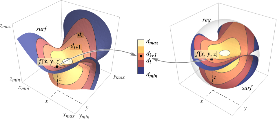
- SliceContourPlot3Dは曲面 surf 上に f[x,y,z]が等しい値 d1,d2等を持つレベル集合に相当する等高線を構築する.デフォルトで,値が diから di+1までの領域が簡単に識別できるように曲線間の領域は陰影付けされる.
- 以下は領域
 を可視化したものである.
- 次の基本的なスライス面 surfiを与えることができる.
-
Automatic スライス面を自動的に決定する 
"CenterPlanes" 中心を通る座標平面 
"BackPlanes" プロットの後ろの座標平面 
"XStackedPlanes"  軸に沿って積み重ねられた座標平面

"YStackedPlanes"  軸に沿って積み重ねられた座標平面

"ZStackedPlanes"  軸に沿って積み重ねられた座標平面

"DiagonalStackedPlanes" 対角上に軸に沿って積み重ねられた座標平面 
"CenterSphere" 中心の球 
"CenterCutSphere" 切り取られたウェッジがある球 
"CenterCutBox" 切り取られた象限があるボックス - SliceContourPlot3D[f,{x,xmin,xmax},…]はSliceContourPlot3D[f,Automatic,{x,xmin,xmax},…]等に等しい.
- 基本的なスライス面には次のパラメータ化を使うことができる.
-
{"XStackedPlanes",n}, n 個の等間隔の平面を生成 {"XStackedPlanes",{x1,x2,…}}  についての平面を生成
{"CenterCutSphere",ϕopen} 視点に面したカット角 ϕopen {"CenterCutSphere",ϕopen,ϕcenter}  平面上の中心角が ϕcenterのカット角 ϕopen
- "YStackedPlanes"および "ZStackedPlanes"は"XStackedPlanes"についての指定に従う.追加的な特徴はスコープの例で示す.
- 次の一般的なスライス面 surfiを使うことができる.
-
expr0 x,y,z による陰的方程式,例:x y z-10 surfaceregion 3Dにおける二次元領域,例:Hyperplane volumeregion surfiが境界面とみなされる3Dにおける三次元領域,例:Cuboid - スライス面 surfiには次のラッパーを使うことができる.
-
Annotation[surf,label] 注釈を与える Button[surf,action] 曲面がクリックされた際に実行する動作を定義 EventHandler[surf,…] 曲面の一般的なイベントハンドラを定義 Hyperlink[surf,uri] 曲面がハイパーリンクとして動作するようにする PopupWindow[surf,cont] 曲面にポップアップウィンドウを付ける StatusArea[surf,label] 曲面上にマウスが来た場合にステータスエリアに表示 Tooltip[surf,label] 曲面に任意のツールチップを付ける - SliceContourPlot3Dには,Graphics3Dと同じオプションに以下の追加・変更を加えたものが使える. [全オプションのリスト]
-
Axes True 軸を描くかどうか BoundaryStyle Automatic 表面の境界にどのようにスタイル付けするか BoxRatios {1,1,1} 境界3Dボックスの比 ClippingStyle None PlotRangeで切り取られた値をどのように描画するか ColorFunction Automatic プロットにどのように彩色するか ColorFunctionScaling True ColorFunctionの引数をスケールするかどうか Contours Automatic どのような等高線あるいは何本の等高線を示すか ContourShading Automatic 等高線間の領域の陰影をどのように付けるか ContourStyle Automatic 等高線のスタイル PerformanceGoal $PerformanceGoal パフォーマンスのどの面について最適化するか PlotLegends None 色勾配の凡例 PlotPoints Automatic 各方向の関数 f およびスライス面 surfiについてのサンプルの初期数 PlotRange {Full,Full,Full,Automatic} 含める f あるいは他の値の範囲 PlotTheme $PlotTheme プロットの全体的なテーマ RegionFunction (True&) 点を含めるかどうかの決め方 ScalingFunctions None 個々の座標のスケール方法 TargetUnits Automatic 使用する所望の単位 WorkingPrecision MachinePrecision 内部計算に使う精度 - ColorFunctionには,デフォルトで,f のスケールされた値が渡される.
- RegionFunctionには,デフォルトで,x,y,z,f が渡される.
- 次は,ScalingFunctionsの可能な設定である.
-
sf f 等高線の値をスケールする {sx,sy,sz} x,y, z の各軸をスケールする {sx,sy,sz,sf} x,y, z の各軸と f 等高線の値をスケールする - 次は,よく使われる組込みのスケーリング関数 s である.
-
"Log" 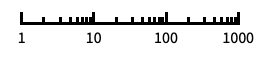
自動的に目盛ラベルを付ける対数スケール "Log10" 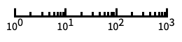
10のベキ乗に目盛を置く,10を底とした対数スケール "SignedLog" 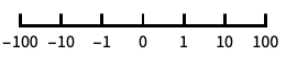
0と負の数を含む対数に似たスケール "Reverse" 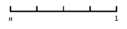
座標の向きを逆にする "Infinite" 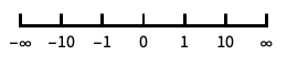
無限スケール
全オプションのリスト
例題
すべて開く すべて閉じる例 (2)

SliceContourPlot3D[Exp[-(x ^ 2 + y ^ 2 + z ^ 2)], "CenterPlanes", {x, -2, 2}, {y, -2, 2}, {z, -2, 2}]
SliceContourPlot3D[Exp[-(x ^ 2 + y ^ 2 + z ^ 2)], x ^ 3 + y ^ 2 - z ^ 2 == 0, {x, -2, 2}, {y, -2, 2}, {z, -2, 2}]スコープ (24)
表面 (9)
Table[SliceContourPlot3D[Sin[x] + y ^ 2 - z ^ 3, sl, {x, -1, 1}, {y, -1, 1}, {z, -1, 1}, PlotLabel -> sl], {sl, {"CenterPlanes", "BackPlanes", "DiagonalStackedPlanes"}}]Table[SliceContourPlot3D[Sin[x] + y ^ 2 - z ^ 3, sl, {x, -1, 1}, {y, -1, 1}, {z, -1, 1}, PlotLabel -> sl], {sl, {"XStackedPlanes", "YStackedPlanes", "ZStackedPlanes"}}]Table[SliceContourPlot3D[Sin[x] + y ^ 2 - z ^ 3, sl, {x, -1, 1}, {y, -1, 1}, {z, -1, 1}, PlotLabel -> sl], {sl, {"CenterSphere", "CenterCutSphere", "CenterCutBox"}}]SliceContourPlot3D[x + y + z, HalfPlane[{{0, 0, 0}, {1, 0, 0}}, {0, 1, 1}], {x, -1, 1}, {y, -1, 1}, {z, -1, 1}]質量プリミティブ上でのプロットはRegionBoundary[reg]上でのプロットに等しい:
SliceContourPlot3D[x + y + z, Cylinder[], {x, -1, 1}, {y, -1, 1}, {z, -1, 1}]
SliceContourPlot3D[Sin[x y z], x ^ 3 + y ^ 2 - z ^ 2 == 0, {x, -2, 2}, {y, -2, 2}, {z, -2, 2}]SliceContourPlot3D[Sin[x y z], {Cylinder[], "BackPlanes"}, {x, -2, 2}, {y, -2, 2}, {z, -2, 2}, Contours -> 3]SliceContourPlot3D[x + y + z, {"XStackedPlanes", 7}, {x, -2, 2}, {y, -2, 2}, {z, -2, 2}]中心が切り取られた表面スライスについて切り取り角度を指定する:
SliceContourPlot3D[Sin[x y z], {"CenterCutSphere", 2Pi / 3}, {x, -2, 2}, {y, -2, 2}, {z, -2, 2}]サンプリング (4)
Contoursを使って等高線数を指定する:
SliceContourPlot3D[x + y + z, "BackPlanes", {x, -2, 2}, {y, -2, 2}, {z, -2, 2}, Contours -> 5]
SliceContourPlot3D[x + y + z, "BackPlanes", {x, -2, 2}, {y, -2, 2}, {z, -2, 2}, Contours -> {-1, 0, 1}]SliceContourPlot3D[Sqrt[x y z], "CenterSphere", {x, -1, 1}, {y, -1, 1}, {z, -1, 1}]RegionFunctionを使ってあいまいなスライスを露出させる:
SliceContourPlot3D[x ^ 2 + y ^ 2 + z ^ 2, "ZStackedPlanes", {x, -2, 2}, {y, -2, 2}, {z, -2, 2}, RegionFunction -> Function[{x, y, z}, x < 0 || y > 0]]領域はConeを含む領域で指定することができる:
SliceContourPlot3D[x + y + z, "CenterPlanes", {x, y, z}∈Cone[]]数式定義領域はImplicitRegionを含んでいる:
ℛ = ImplicitRegion[(x ^ 2 + (9 / 4)y ^ 2 + z ^ 2 - 1) ^ 3 - x ^ 2z ^ 3 - (9 / 80)y ^ 2z ^ 3 <= 0, {{x, -1.2, 1.2}, {y, -0.7, 0.7}, {z, -1, 1.3}}];SliceContourPlot3D[x + y + z, "CenterPlanes", {x, y, z}∈ℛ]BoundaryMeshRegionを含む,メッシュに基づいた領域:
ℛ = ConvexHullMesh[RandomReal[1, {25, 3}]]SliceContourPlot3D[x + y + z, "CenterPlanes", {x, y, z}∈ℛ]プレゼンテーション (11)
PlotThemeを使って全体的なスタイルを即座に得る:
Table[SliceContourPlot3D[x ^ 2 + y ^ 2 + z ^ 2, "CenterPlanes", {x, -1, 1}, {y, -1, 1}, {z, -1, 1}, PlotLabel -> t, PlotTheme -> t], {t, {"Minimal", "Scientific", "Marketing"}}]PlotLegendsを使ってさまざまな値についての色の棒を得る:
SliceContourPlot3D[x ^ 2 + y ^ 2 + z ^ 2, "CenterPlanes", {x, -1, 1}, {y, -1, 1}, {z, -1, 1}, PlotLegends -> Automatic]Axesで軸の表示を制御する:
Table[SliceContourPlot3D[x + y + z, "CenterPlanes", {x, -2, 2}, {y, -2, 2}, {z, -2, 2}, PlotLabel -> a, Axes -> a], {a, {True, False, {True, False, True}}}]AxesLabelを使って軸に,PlotLabelを使ってプロット全体にラベルを付ける:
SliceContourPlot3D[x ^ 2 + y ^ 2 + z ^ 2, "CenterPlanes", {x, -2, 2}, {y, -2, 2}, {z, -2, 2}, Ticks -> None, AxesLabel -> {x, y, z}, PlotLabel -> x ^ 2 + y ^ 2 + z ^ 2]ColorFunctionで関数値によってプロットに色付けする:
Table[SliceContourPlot3D[Sin[3x y z], "ZStackedPlanes", {x, -1, 1}, {y, -1, 1}, {z, -1, 1}, PlotLabel -> c, ColorFunction -> c], {c, {Hue, "BlueGreenYellow"}}]ContourShadingで等高線の間の領域にスタイル付けする:
SliceContourPlot3D[Exp[-(x ^ 2 + y ^ 2 + z ^ 2)], "CenterPlanes", {x, -1, 1}, {y, -1, 1}, {z, -1, 1}, Contours -> 9, BoundaryStyle -> None, ContourShading -> {Orange, None, Blue}]ContourStyleを使って等高線にスタイルを付ける:
SliceContourPlot3D[x ^ 4 + y ^ 4 + z ^ 4 - x ^ 2 - y ^ 2 - z ^ 2, "CenterSphere", {x, -1, 1}, {y, -1, 1}, {z, -1, 1}, ContourStyle -> Dotted]BoundaryStyleでスライス面の境界にスタイルを付ける:
SliceContourPlot3D[Exp[-(x ^ 2 + y ^ 2 + z ^ 2)], "CenterPlanes", {x, -2, 2}, {y, -2, 2}, {z, -2, 2}, BoundaryStyle -> Gray]TargetUnitsで可視化に使う単位を指定する:
SliceContourPlot3D[Quantity[-(x ^ 2 + y ^ 2 + z ^ 2), "kg/m^3"], "CenterPlanes", {x, -2, 2}, {y, -2, 2}, {z, -2, 2}, AxesLabel -> Automatic, PlotLegends -> Automatic, TargetUnits -> {"Feet", "Feet", "Feet", "g/ft^3"}]
SliceContourPlot3D[x + y + z, {x, 1, 100}, {y, 1, 100}, {z, 1, 100}, ScalingFunctions -> {"Log", None, None}]
SliceContourPlot3D[x + y + z, {x, 1, 100}, {y, 1, 100}, {z, 1, 100}, ScalingFunctions -> {None, None, "Reverse"}]オプション (69)
Axes (3)
SliceContourPlot3D[-(x ^ 2 + y ^ 2 + z ^ 2), "CenterPlanes", {x, -2, 2}, {y, -2, 2}, {z, -2, 2}]SliceContourPlot3D[-(x ^ 2 + y ^ 2 + z ^ 2), "CenterPlanes", {x, -2, 2}, {y, -2, 2}, {z, -2, 2}, Axes -> False]{SliceContourPlot3D[-(x ^ 2 + y ^ 2 + z ^ 2), "CenterPlanes", {x, -2, 2}, {y, -2, 2}, {z, -2, 2}, Axes -> {False, False, True}], SliceContourPlot3D[-(x ^ 2 + y ^ 2 + z ^ 2), "CenterPlanes", {x, -2, 2}, {y, -2, 2}, {z, -2, 2}, Axes -> {False, True, False}], SliceContourPlot3D[-(x ^ 2 + y ^ 2 + z ^ 2), "CenterPlanes", {x, -2, 2}, {y, -2, 2}, {z, -2, 2}, Axes -> {True, False, False}]}AxesLabel (4)
SliceContourPlot3D[-(x ^ 2 + y ^ 2 + z ^ 2), "CenterPlanes", {x, -2, 2}, {y, -2, 2}, {z, -2, 2}]
SliceContourPlot3D[-(x ^ 2 + y ^ 2 + z ^ 2), "CenterPlanes", {x, -2, 2}, {y, -2, 2}, {z, -2, 2}, AxesLabel -> "height"]SliceContourPlot3D[-(x ^ 2 + y ^ 2 + z ^ 2), "CenterPlanes", {x, -2, 2}, {y, -2, 2}, {z, -2, 2}, AxesLabel -> {"width", "depth", "height"}]SliceContourPlot3Dで指定された変数に基づくラベルを使う:
SliceContourPlot3D[-(x ^ 2 + y ^ 2 + z ^ 2), "CenterPlanes", {x, -2, 2}, {y, -2, 2}, {z, -2, 2}, AxesLabel -> Automatic]AxesOrigin (2)
AxesStyle (3)
SliceContourPlot3D[-(x ^ 2 + y ^ 2 + z ^ 2), "CenterPlanes", {x, -2, 2}, {y, -2, 2}, {z, -2, 2}, AxesStyle -> Red]SliceContourPlot3D[-(x ^ 2 + y ^ 2 + z ^ 2), "CenterPlanes", {x, -2, 2}, {y, -2, 2}, {z, -2, 2}, AxesStyle -> {{Thick, Brown}, {Thick, Blue}, {Thick, Green}}]SliceContourPlot3D[-(x ^ 2 + y ^ 2 + z ^ 2), "CenterPlanes", {x, -2, 2}, {y, -2, 2}, {z, -2, 2}, AxesStyle -> Green, TicksStyle -> Blue]BoundaryStyle (1)
BoundaryStyleでスライス面の境界にスタイル付けする:
SliceContourPlot3D[-(x ^ 2 + y ^ 2 + z ^ 2), "CenterPlanes", {x, -2, 2}, {y, -2, 2}, {z, -2, 2}, BoundaryStyle -> Gray]BoxRatios (3)
SliceContourPlot3D[x y z, "CenterSphere", {x, 0, 1}, {y, 0, 1}, {z, -1, 2}]BoxRatios->Automaticを使って3D座標値の自然なスケールを示す:
SliceContourPlot3D[x y z, "CenterSphere", {x, 0, 1}, {y, 0, 1}, {z, -1, 2}, BoxRatios -> Automatic]SliceContourPlot3D[x y z, "CenterSphere", {x, 0, 1}, {y, 0, 1}, {z, -1, 2}, BoxRatios -> {1, 2, 2}]ClippingStyle (2)
SliceContourPlot3D[Exp[-(x ^ 2 + y ^ 2 + z ^ 2)], "CenterPlanes", {x, -2, 2}, {y, -2, 2}, {z, -2, 2}, PlotRange -> {0.09, 0.72}, ClippingStyle -> {Gray, Green}]Noneを使って切り取られた領域を削除する:
SliceContourPlot3D[Exp[-(x ^ 2 + y ^ 2 + z ^ 2)], "CenterPlanes", {x, -2, 2}, {y, -2, 2}, {z, -2, 2}, PlotRange -> {0.09, 0.72}, ClippingStyle -> None]ColorFunction (3)

SliceContourPlot3D[x + y z, "ZStackedPlanes", {x, -1, 1}, {y, -1, 1}, {z, -1, 1}, ColorFunction -> Hue]SliceContourPlot3D[x ^ 2 + y ^ 2 + z ^ 2, "CenterPlanes", {x, -2, 2}, {y, -2, 2}, {z, -2, 2}, ColorFunction -> "IslandColors"]
SliceContourPlot3D[Sin[2 x y z], "ZStackedPlanes", {x, -2, 2}, {y, -2, 2}, {z, -2, 2}, ColorFunction -> Function[f, If[f < 0, Red, Green]],
	ColorFunctionScaling -> False, Contours -> 3]
ColorFunctionScaling (2)
SliceContourPlot3D[x y z, "BackPlanes", {x, -2, 2}, {y, -2, 2}, {z, -2, 2}, ColorFunction -> Hue]ColorFunctionScalingFalseを使ってスケールされていない値を得る:
SliceContourPlot3D[x y z, "BackPlanes", {x, -2, 2}, {y, -2, 2}, {z, -2, 2}, ColorFunction -> (If[# <= 0, Red, Green]&), ColorFunctionScaling -> False]Contours (4)
SliceContourPlot3D[x ^ 3 + y ^ 2 - z ^ 2, "BackPlanes", {x, -2, 2}, {y, -2, 2}, {z, -2, 2}, Contours -> 5]SliceContourPlot3D[x ^ 3 + y ^ 2 - z ^ 2, "BackPlanes", {x, -2, 2}, {y, -2, 2}, {z, -2, 2}, Contours -> Automatic]SliceContourPlot3D[x ^ 3 + y ^ 2 - z ^ 2, "BackPlanes", {x, -2, 2}, {y, -2, 2}, {z, -2, 2}, Contours -> {-1, 1}]SliceContourPlot3D[x ^ 3 + y ^ 2 - z ^ 2, "BackPlanes", {x, -2, 2}, {y, -2, 2}, {z, -2, 2}, Contours -> {{-1, Green}, {1, Dashed}}]ContourStyle (1)
ContourShading (4)
ContourShadingAutomaticは,ColorFunctionから等高線領域の陰影付けを計算する:
SliceContourPlot3D[Exp[-(x ^ 2 + y ^ 2 + z ^ 2)], "CenterPlanes", {x, -1, 1}, {y, -1, 1}, {z, -1, 1}, Contours -> 9, BoundaryStyle -> None, ContourShading -> Automatic, ColorFunction -> "BrightBands"]SliceContourPlot3D[Exp[-(x ^ 2 + y ^ 2 + z ^ 2)], "CenterPlanes", {x, -1, 1}, {y, -1, 1}, {z, -1, 1}, Contours -> 9, BoundaryStyle -> None, ContourShading -> {Orange, Blue}]SliceContourPlot3D[Exp[-(x ^ 2 + y ^ 2 + z ^ 2)], "CenterPlanes", {x, -1, 1}, {y, -1, 1}, {z, -1, 1}, Contours -> 9, BoundaryStyle -> None, ContourShading -> {Orange, None, Blue}]SliceContourPlot3D[Exp[-(x ^ 2 + y ^ 2 + z ^ 2)], "CenterPlanes", {x, -1, 1}, {y, -1, 1}, {z, -1, 1}, Contours -> 9, BoundaryStyle -> None, ContourShading -> None]ImageSize (7)
Tiny,Small,Medium,Largeのような名前付きのサイズを使う:
{SliceContourPlot3D[-(x ^ 2 + y ^ 2 + z ^ 2), "CenterPlanes", {x, -2, 2}, {y, -2, 2}, {z, -2, 2}, ImageSize -> Tiny], SliceContourPlot3D[-(x ^ 2 + y ^ 2 + z ^ 2), "CenterPlanes", {x, -2, 2}, {y, -2, 2}, {z, -2, 2}, ImageSize -> Small]}{SliceContourPlot3D[-(x ^ 2 + y ^ 2 + z ^ 2), "CenterPlanes", {x, -2, 2}, {y, -2, 2}, {z, -2, 2}, ImageSize -> 150], SliceContourPlot3D[-(x ^ 2 + y ^ 2 + z ^ 2), "CenterPlanes", {x, -2, 2}, {y, -2, 2}, {z, -2, 2}, AspectRatio -> 1.5, ImageSize -> 150]}{SliceContourPlot3D[-(x ^ 2 + y ^ 2 + z ^ 2), "CenterPlanes", {x, -2, 2}, {y, -2, 2}, {z, -2, 2}, ImageSize -> {Automatic, 150}], SliceContourPlot3D[-(x ^ 2 + y ^ 2 + z ^ 2), "CenterPlanes", {x, -2, 2}, {y, -2, 2}, {z, -2, 2}, AspectRatio -> 2, ImageSize -> {Automatic, 150}]}{SliceContourPlot3D[-(x ^ 2 + y ^ 2 + z ^ 2), "CenterPlanes", {x, -2, 2}, {y, -2, 2}, {z, -2, 2}, ImageSize -> UpTo[200]], SliceContourPlot3D[-(x ^ 2 + y ^ 2 + z ^ 2), "CenterPlanes", {x, -2, 2}, {y, -2, 2}, {z, -2, 2}, AspectRatio -> 2, ImageSize -> UpTo[200]]}グラフィックスの幅と高さを指定して,必要な場合はスペースで充填する:
SliceContourPlot3D[-(x ^ 2 + y ^ 2 + z ^ 2), "CenterPlanes", {x, -2, 2}, {y, -2, 2}, {z, -2, 2}, ImageSize -> {200, 250}, Background -> StandardGray]AspectRatioFullと設定すると,使用可能なスペースが塗り潰される:
SliceContourPlot3D[-(x ^ 2 + y ^ 2 + z ^ 2), "CenterPlanes", {x, -2, 2}, {y, -2, 2}, {z, -2, 2}, AspectRatio -> Full, ImageSize -> {200, 250}, Background -> StandardGray]{SliceContourPlot3D[-(x ^ 2 + y ^ 2 + z ^ 2), "CenterPlanes", {x, -2, 2}, {y, -2, 2}, {z, -2, 2}, ImageSize -> {UpTo[150], UpTo[100]}], SliceContourPlot3D[-(x ^ 2 + y ^ 2 + z ^ 2), "CenterPlanes", {x, -2, 2}, {y, -2, 2}, {z, -2, 2}, AspectRatio -> 2, ImageSize -> {UpTo[150], UpTo[100]}]}ImageSizeFullを使ってオブジェクト内の使用可能なスペースを塗り潰す:
Framed[Pane[SliceContourPlot3D[-(x ^ 2 + y ^ 2 + z ^ 2), "CenterPlanes", {x, -2, 2}, {y, -2, 2}, {z, -2, 2}, ImageSize -> Full, Background -> StandardGray], {200, 200}]]Framed[Pane[SliceContourPlot3D[-(x ^ 2 + y ^ 2 + z ^ 2), "CenterPlanes", {x, -2, 2}, {y, -2, 2}, {z, -2, 2}, AspectRatio -> Full, ImageSize -> {Scaled[0.5], Scaled[0.5]}, Background -> StandardGray], {200, 200}]]PerformanceGoal (2)
Timing[SliceContourPlot3D[x ^ 2 + y ^ 2 + z ^ 2, "CenterPlanes", {x, -2, 2}, {y, -2, 2}, {z, -2, 2}, PerformanceGoal -> "Quality"]]Timing[SliceContourPlot3D[x ^ 2 + y ^ 2 + z ^ 2, "CenterPlanes", {x, -2, 2}, {y, -2, 2}, {z, -2, 2}, PerformanceGoal -> "Speed"]]PlotLegends (4)
SliceContourPlot3D[Sin[x]Sin[y]Sin[z], "BackPlanes", {x, -1, 1}, {y, -1, 1}, {z, -1, 1}, PlotLegends -> Automatic]PlotLegendsは,自動的にContoursとContourShadingの値を拾う:
SliceContourPlot3D[Sin[x]Sin[y]Sin[z], "BackPlanes", {x, -2, 2}, {y, -2, 2}, {z, -2, 2}, ContourShading -> {Red, Green, Blue, Yellow}, Contours -> 3, PlotLegends -> Automatic]ContourShadingAutomaticと設定すると,色はColorFunctionから取られる:
SliceContourPlot3D[Sin[x]Sin[y]Sin[z], "BackPlanes", {x, -2, 2}, {y, -2, 2}, {z, -2, 2}, ColorFunction -> "Rainbow", PlotLegends -> Automatic]Placedを使って凡例の配置を制御する:
SliceContourPlot3D[Sin[x]Sin[y]Sin[z], "BackPlanes", {x, -2, 2}, {y, -2, 2}, {z, -2, 2}, PlotLegends -> Placed[Automatic, Above]]PlotPoints (1)
PlotRange (3)
デフォルトでAll等高線が示される:
SliceContourPlot3D[Sin[3x y z], "CenterSphere", {x, -1, 1}, {y, -1, 1}, {z, -1, 1}]SliceContourPlot3D[Sin[3x y z], "CenterSphere", {x, -1, 1}, {y, -1, 1}, {z, -1, 1}, PlotRange -> {All, All, {0, 2}}, BoxRatios -> Automatic]SliceContourPlot3D[x + y + z, "CenterPlanes", {x, -1, 1}, {y, -1, 1}, {z, -1, 1}, PlotRange -> {0, 2}]SliceContourPlot3D[x + y + z, "CenterPlanes", {x, -1, 1}, {y, -1, 1}, {z, -1, 1}, PlotRange -> {All, All, All, {0, 2}}]PlotTheme (3)
SliceContourPlot3D[-(x ^ 2 + y ^ 2 + z ^ 2), "CenterPlanes", {x, -2, 2}, {y, -2, 2}, {z, -2, 2}, PlotTheme -> "Detailed"]任意のオプション設定でPlotThemeスタイルを無効にする.この場合は面格子が除去される:
SliceContourPlot3D[-(x ^ 2 + y ^ 2 + z ^ 2), "CenterPlanes", {x, -2, 2}, {y, -2, 2}, {z, -2, 2}, PlotTheme -> "Detailed", FaceGrids -> None]Table[SliceContourPlot3D[x ^ 2 + y ^ 2 + z ^ 2, "CenterPlanes", {x, -2, 2}, {y, -2, 2}, {z, -2, 2}, PlotLabel -> t, PlotTheme -> t, ImageSize -> 130], {t, {"Scientific", "Monochrome", "Minimal", "Web", "Working", "Classic", "Business", "Marketing", "Detailed"}}]RegionFunction (2)


SliceContourPlot3D[x ^ 2 + y ^ 2 + z ^ 2, "ZStackedPlanes", {x, -2, 2}, {y, -2, 2}, {z, -2, 2}, RegionFunction -> Function[{x, y, z, f}, x < 0 || y > 0]]
SliceContourPlot3D[x ^ 2 + y ^ 2 + z ^ 2, "CenterPlanes", {x, -2, 2}, {y, -2, 2}, {z, -2, 2}, RegionFunction -> Function[{x, y, z, f}, f > 2]]ScalingFunctions (5)
SliceContourPlot3D[x + y + z, {x, 1, 20}, {y, 1, 20}, {z, 1, 20}]
SliceContourPlot3D[x + y + z, {x, 1, 50}, {y, 1, 50}, {z, 1, 50}, ScalingFunctions -> {"Log", None, None}]ScalingFunctionsを使って  方向の座標の向きが逆になるようにスケールする:
SliceContourPlot3D[x + y + z, {x, 1, 100}, {y, 1, 100}, {z, 1, 100}, ScalingFunctions -> {None, None, "Reverse"}]SliceContourPlot3D[x + y + z, {x, 1, 100}, {y, 1, 100}, {z, 1, 100}, ScalingFunctions -> {None, None, {-Log[#]&, Exp[-#]&}}]境界ボックスと相対的に定義されたスライス表面はスケーリング関数の影響を受けない:
SliceContourPlot3D[x + y + z, "CenterCutSphere", {x, 1, 100}, {y, 1, 100}, {z, 1, 100}, ScalingFunctions -> {None, None, "Log"}]Ticks (6)
SliceContourPlot3D[Exp[-(x ^ 2 + y ^ 2 + z ^ 2)], "CenterPlanes", {x, -2, 2}, {y, -2, 2}, {z, -2, 2}]SliceContourPlot3D[Exp[-(x ^ 2 + y ^ 2 + z ^ 2)], "CenterPlanes", {x, -2, 2}, {y, -2, 2}, {z, -2, 2}, Ticks -> None]SliceContourPlot3D[Exp[-(x ^ 2 + y ^ 2 + z ^ 2)], "CenterPlanes", {x, -2, 2}, {y, -2, 2}, {z, -2, 2}, Ticks -> {{-1.5, 0, 1.5}, {-1.5, 0, 1.5}, {-1.5, 0, 1.5}}]SliceContourPlot3D[Exp[-(x ^ 2 + y ^ 2 + z ^ 2)], "CenterPlanes", {x, -2, 2}, {y, -2, 2}, {z, -2, 2}, Ticks -> {{{-1.5, -a}, {0, 0}, {1.5, a}}, {{-1.5, -a}, {0, 0}, {1.5, a}}, {{-1.5, -a}, {0, 0}, {1.5, a}}}]SliceContourPlot3D[Exp[-(x ^ 2 + y ^ 2 + z ^ 2)], "CenterPlanes", {x, -2, 2}, {y, -2, 2}, {z, -2, 2}, Ticks -> {{{-1.5, -a, .1}, {0, 0, .1}, {1.5, a, .1}}, {{-1.5, -a, .05}, {0, 0, .05}, {1.5, a, .05}}, {{-1.5, -a, .15}, {0, 0, .15}, {1.5, a, .15}}}]SliceContourPlot3D[Exp[-(x ^ 2 + y ^ 2 + z ^ 2)], "CenterPlanes", {x, -2, 2}, {y, -2, 2}, {z, -2, 2}, Ticks -> {{{-1.5, -a, .1, Directive[Red, Dashed, Thick]}, {0, 0, .1, Directive[Red, Dashed]}, {1.5, a, .1, Directive[Red]}}, {{-1.5, -a, .05, Directive[Blue, Dashed, Thick]}, {0, 0, .05, Directive[Blue, Dashed]}, {1.5, a, .05, Directive[Blue]}}, {{-1.5, -a, .15, Directive[Darker@Green, Dashed, Thick]}, {0, 0, .15, Directive[Darker@Green, Dashed]}, {1.5, a, .15, Directive[Darker@Green]}}}]TicksStyle (3)
デフォルトで,目盛と目盛ラベルには軸と同じスタイルが使われる:
SliceContourPlot3D[Exp[-(x ^ 2 + y ^ 2 + z ^ 2)], "CenterPlanes", {x, -2, 2}, {y, -2, 2}, {z, -2, 2}, AxesStyle -> Directive[Bold, Red]]SliceContourPlot3D[Exp[-(x ^ 2 + y ^ 2 + z ^ 2)], "CenterPlanes", {x, -2, 2}, {y, -2, 2}, {z, -2, 2}, TicksStyle -> Directive[Bold, Red]]SliceContourPlot3D[Exp[-(x ^ 2 + y ^ 2 + z ^ 2)], "CenterPlanes", {x, -2, 2}, {y, -2, 2}, {z, -2, 2}, TicksStyle -> {Directive[Green, Bold], Directive[Bold, Red], Directive[Bold, Blue]}]アプリケーション (17)
初等関数 (4)

SliceContourPlot3D[x, "BackPlanes", {x, -2, 2}, {y, -2, 2}, {z, -2, 2}]

{SliceContourPlot3D[y, "BackPlanes", {x, -2, 2}, {y, -2, 2}, {z, -2, 2}],
	SliceContourPlot3D[z, "BackPlanes", {x, -2, 2}, {y, -2, 2}, {z, -2, 2}]}

{SliceContourPlot3D[x + y, "BackPlanes", {x, -2, 2}, {y, -2, 2}, {z, -2, 2}],
	SliceContourPlot3D[y + z, "BackPlanes", {x, -2, 2}, {y, -2, 2}, {z, -2, 2}]}

{SliceContourPlot3D[x + y + z, "BackPlanes", {x, -2, 2}, {y, -2, 2}, {z, -2, 2}],
	SliceContourPlot3D[x - y + z, "BackPlanes", {x, -2, 2}, {y, -2, 2}, {z, -2, 2}]}

{SliceContourPlot3D[x ^ 2 + y ^ 2, "CenterPlanes", {x, -2, 2}, {y, -2, 2}, {z, -2, 2}, Contours -> 5], SliceContourPlot3D[y ^ 2 + z ^ 2, "CenterPlanes", {x, -2, 2}, {y, -2, 2}, {z, -2, 2}, Contours -> 5]}

{SliceContourPlot3D[x ^ 2 + y ^ 2 + z ^ 2, "CenterPlanes", {x, -2, 2}, {y, -2, 2}, {z, -2, 2}, Contours -> 5], SliceContourPlot3D[x ^ 2 + y ^ 2 + 2z ^ 2, "CenterPlanes", {x, -2, 2}, {y, -2, 2}, {z, -2, 2}, Contours -> 5]}
surf = {{"XStackedPlanes", {-0.5, 0.5}}, {"ZStackedPlanes", {-0.5, 0.5}}};SliceContourPlot3D[Sin[π x]Sin[π y]Sin[π z], surf, {x, -1, 1}, {y, -1, 1}, {z, -1, 1}, Contours -> 5]

{SliceContourPlot3D[Sin[π x]Sin[π (y + z)], surf, {x, -1, 1}, {y, -1, 1}, {z, -1, 1}, Contours -> 5], SliceContourPlot3D[Sin[π (x + y)]Sin[π z], surf, {x, -1, 1}, {y, -1, 1}, {z, -1, 1}, Contours -> 5]}
SliceContourPlot3D[Sin[π (x + y + z)], surf, {x, -1, 1}, {y, -1, 1}, {z, -1, 1}, Contours -> 5]
f = Exp[-Norm[{x, y, z} - {-1, -1, -1}]^2] + Exp[-Norm[{x, y, z} - {1, 1, 1}]^2];SliceContourPlot3D[f, {{"XStackedPlanes", {1, -1}}, {"YStackedPlanes", {1, -1}}, {"ZStackedPlanes", {-1, 1}}}, {x, -3, 3}, {y, -3, 3}, {z, -3, 3}, Contours -> 5, PlotRange -> {0.1, 1.1}]
f = Sum[Exp[-2Norm[{x, y, z} - pi]^2], {pi, RandomPoint[Cuboid[{-1, -1, -1}, {1, 1, 1}], 10]}];SliceContourPlot3D[f, "CenterPlanes", {x, -3, 3}, {y, -3, 3}, {z, -3, 3}, Contours -> 5, PlotRange -> {0.1, 4}]分布関数 (6)
𝒟 = MultinormalDistribution[{0, 0, 0}, {{1, 0.5, 0}, {0.5, 1, 0}, {0, 0, 1}}];
f = PDF[𝒟, {x, y, z}];d = SliceContourPlot3D[f, "CenterPlanes", {x, -2, 2}, {y, -2, 2}, {z, -2, 2}, ColorFunction -> (ColorData["SunsetColors"][1 - #]&)]pts = RandomVariate[𝒟, 10 ^ 4];Show[d, Graphics3D[{Green, AbsolutePointSize[1], Point[pts]}]]分布のCDFをプロットする:
𝒟 = MultinormalDistribution[{0, 0, 0}, {{1, 0.5, 0}, {0.5, 1, 0}, {0, 0, 1}}];
cdf = CDF[𝒟, {x, y, z}];SliceContourPlot3D[cdf, {x == y, x == 2, y == 2}, {x, -2, 2}, {y, -2, 2}, {z, -1, 2}, Contours -> 5, PlotRange -> {0.1, 1}]sf = SurvivalFunction[𝒟, {x, y, z}];SliceContourPlot3D[sf, {x == y, x == -2, y == -2}, {x, -2, 2}, {y, -2, 2}, {z, -1, 2}, Contours -> 5, PlotRange -> {0.1, 1}]hf = HazardFunction[𝒟, {x, y, z}];SliceContourPlot3D[hf, {x == y, x == 2, y == 2}, {x, -2, 2}, {y, -2, 2}, {z, -1, 2}, Contours -> 5, PlotRange -> {1, 8}]MultinormalDistributionのCorrelation母数を調べる.ρabは a と b の間の相関である:
cov[{σx_, σy_, σz_}, {ρxy_, ρyz_, ρxz_}] := {{σx^2, σx σy ρxy, σx σz ρxz}, {σx σy ρxy, σy^2, σy σz ρyz}, {σx σz ρxz, σy σz ρyz, σz^2}};Σ = cov[{1, 1, 1}, {0.5, 0, 0}];
f = PDF[MultinormalDistribution[{0, 0, 0}, Σ], {x, y, z}];SliceContourPlot3D[f, "CenterPlanes", {x, -2, 2}, {y, -2, 2}, {z, -2, 2}, ColorFunction -> (ColorData["SunsetColors"][1 - #]&)]Σ = cov[{1, 1, 1}, {0, 0.5, 0}];
f = PDF[MultinormalDistribution[{0, 0, 0}, Σ], {x, y, z}];SliceContourPlot3D[f, "CenterPlanes", {x, -2, 2}, {y, -2, 2}, {z, -2, 2}, ColorFunction -> (ColorData["SunsetColors"][1 - #]&)]y と z のみの間の相関.ただし,z 成分のより大きい分散  :
Σ = cov[{1, 1, 2}, {0, 0.5, 0}];
f = PDF[MultinormalDistribution[{0, 0, 0}, Σ], {x, y, z}];SliceContourPlot3D[f, "CenterPlanes", {x, -2, 2}, {y, -2, 2}, {z, -4, 4}, BoxRatios -> Automatic, ColorFunction -> (ColorData["SunsetColors"][1 - #]&)]ProductDistributionのPDFを可視化する:
𝒟 = ProductDistribution[{NormalDistribution[0, 1], 3}];
f = PDF[𝒟, {x, y, z}]SliceContourPlot3D[f, "CenterPlanes", {x, -2, 2}, {y, -2, 2}, {z, -2, 2}, ColorFunction -> (ColorData["SunsetColors"][1 - #]&)]𝒟 = ProductDistribution[NormalDistribution[], LaplaceDistribution[], WeibullDistribution[1, 1]];
f = PDF[𝒟, {x, y, z}]SliceContourPlot3D[f, {{"XStackedPlanes", {0}}, {"YStackedPlanes", {0}}, {"ZStackedPlanes", {0}}}, {x, -2, 2}, {y, -2, 2}, {z, 0, 2}, Contours -> 5, ColorFunction -> (ColorData["SunsetColors"][1 - #]&)]𝒟 = ProductDistribution[BinormalDistribution[1 / 2], ExponentialDistribution[3]];
f = PDF[𝒟, {x, y, z}]SliceContourPlot3D[f, {x == y, x == -y, z == 0}, {x, -2, 2}, {y, -2, 2}, {z, 0, 1}, ColorFunction -> (ColorData["SunsetColors"][1 - #]&)]CopulaDistributionのPDFをプロットする:
𝒟 = CopulaDistribution[{"Frank", 1}, {GammaDistribution[3, 2 / 3], ExponentialDistribution[2], NormalDistribution[]}];
f = PDF[𝒟, {x, y, z}]SliceContourPlot3D[f, {y == 0, z == 0, {"YStackedPlanes", 5}}, {x, 0, 6}, {y, 0, 1.1}, {z, -3, 3}, Contours -> 7, PlotRange -> {0.1, 0.4}]data = RandomVariate[NormalDistribution[], {10 ^ 4, 3}];
f = PDF[SmoothKernelDistribution[data], {x, y, z}];SliceContourPlot3D[f, "CenterPlanes", {x, -3, 3}, {y, -3, 3}, {z, -3, 3}, Contours -> 7, PlotRange -> {0.01, 0.1}]ポテンシャル関数と波動関数 (4)
f = (((x y) Exp[I ((6π/5) - π Sqrt[x^2 + y^2 + z^2])]) (-1 + 2 I + (3 + I/Sqrt[x^2 + y^2 + z^2]))/(x^2 + y^2 + z^2) Sqrt[x^2 + y^2 + z^2]);SliceContourPlot3D[Arg[f], Abs[f] == (Abs[f] /. {x -> 0.2, y -> 0.1, z -> 0.1}), {x, -.25, .25}, {y, -.25, .25}, {z, -.25, .25}, Contours -> {0}]
SliceContourPlot3D[Abs[f], {"ZStackedPlanes", 20}, {x, -.25, .25}, {y, -.25, .25}, {z, -.25, .25}, Contours -> {17, 21}, ContourShading -> Red, ClippingStyle -> None, PlotRange -> {All, All, All, {17, 21}}, BoundaryStyle -> None]

f = Sum[Cos[10 Norm[{x, y, z} - {Sin[θ], Cos[θ], 0}]], {θ, 0, 2 π - (2 π/3), (2 π/3)}]SliceContourPlot3D[f, "CenterPlanes",
{x, -2, 2}, {y, -2, 2}, {z, -2, 2}, Contours -> 3, PlotTheme -> "Minimal"]


a0 = Quantity["BohrRadius"] / Quantity["Meters"]ψ[{n_, l_, m_}, {r_, θ_, ϕ_}] := With[{ρ = 2r / (n a0)}, Sqrt[((2/n a0))^3((n - l - 1)!/2n(n + l)!)]Exp[-ρ / 2]ρ^lLaguerreL[n - l - 1, 2l + 1, ρ]SphericalHarmonicY[l, m, θ, ϕ]]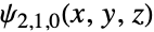
SliceContourPlot3D[(Abs@ψ[{2, 1, 0}, {Sqrt[x^2 + y^2 + z^2], ArcTan[z, Sqrt[x^2 + y^2]], ArcTan[x, y]}])^2, "CenterCutSphere", {x, -5 a0, 5 a0}, {y, -5 a0, 5 a0}, {z, -5 a0, 5 a0}, Contours -> 5, PlotLegends -> Automatic]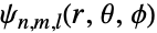
Grid@(Flatten /@ Table[SliceContourPlot3D[(Abs@ψ[{n, l, m}, {Sqrt[x^2 + y^2 + z^2], ArcTan[z, Sqrt[x^2 + y^2]], ArcTan[x, y]}])^2, "CenterCutSphere", {x, -5 a0, 5 a0}, {y, -5 a0, 5 a0}, {z, -5 a0, 5 a0}, Contours -> 5, PlotLabel -> {n, l, m}, Axes -> None, Boxed -> False, ImageSize -> Tiny], {n, 1, 3}, {l, 0, n - 1}, {m, -l, l}])

ElectroStaticPotential[ql_, pl_, r_] := Sum[ (ql[[i]]/Norm[r - pl[[i]]]), {i, Length[ql]}]ElectroStaticPotential[{Subscript[q, 1], Subscript[q, 2]}, {{Subscript[x, 1], Subscript[y, 1], Subscript[z, 1]}, {Subscript[x, 2], Subscript[y, 2], Subscript[z, 2]}}, {x, y, z}]//TraditionalForm

p1 = SliceContourPlot3D[Evaluate[Clip@ElectroStaticPotential[{1, -1}, {{-1, -1, 0}, {1, 1, 0}}, {x, y, z}]], "ZStackedPlanes", {x, -2, 2}, {y, -2, 2}, {z, -2, 2}, ColorFunction -> "Rainbow", PlotLegends -> Automatic, PlotPoints -> 50]p2 = ContourPlot3D[Evaluate[ElectroStaticPotential[{1, -1}, {{-1, -1, 0}, {1, 1, 0}}, {x, y, z}]], {x, -2, 2}, {y, -2, 2}, {z, -2, 2}, Contours -> {-0.3, 0, 0.3}, Mesh -> None, ContourStyle -> Opacity[0.8]]Show[p1, p2]偏微分方程式 (3)
時間が z 軸に沿って表現された周期境界条件を持つ,2つの空間次元の非線形sine-Gordon方程式を可視化する:
L = 4;
usol = NDSolveValue[{D[u[t, x, y], t, t] == D[u[t, x, y], x, x] + D[u[t, x, y], y, y] + Sin[u[t, x, y]], u[t, -L, y] == u[t, L, y], u[t, x, -L] == u[t, x, L], u[0, x, y] == Exp[-(x ^ 2 + y ^ 2)], Derivative[1, 0, 0][u][0, x, y] == 0}, u, {t, 0, L / 2}, {x, -L, L}, {y, -L, L}]SliceContourPlot3D[usol[t, x, y], "CenterCutSphere", {x, -L, L}, {y, -L, L}, {t, 0, L / 2}, AxesLabel -> Automatic, PlotLegends -> Automatic]Wolframの非線形波動方程式を時間が z 軸に沿って表現された2つの空間次元で可視化する:
usol = NDSolveValue[{D[u[t, x, y], t, t] == D[u[t, x, y], x, x] + D[u[t, x, y], y, y] / 2 + (1 - u[t, x, y] ^ 2)(1 + 2u[t, x, y]), u[0, x, y] == E^-(x^2 + y^2), u[t, -5, y] == u[t, 5, y], u[t, x, -5] == u[t, x, 5], u^(1, 0, 0)[0, x, y] == 0}, u, {t, 0, 4}, {x, -5, 5}, {y, -5, 5}]SliceContourPlot3D[usol[t, x, y], "CenterCutSphere", {x, -5, 5}, {y, -5, 5}, {t, 1, 4}, AxesLabel -> Automatic, ColorFunction -> "BrightBands", PlotLegends -> Automatic]3D偏微分方程式の解(この場合はBall上のポアソン方程式とディリクレ境界条)を可視化する:
usol = NDSolveValue[{Subsuperscript[∇, {x, y, z}, 2]u[x, y, z] == 1, DirichletCondition[u[x, y, z] == x y z, True]}, u, {x, y, z}∈Ball[]]SliceContourPlot3D[usol[x, y, z], "XStackedPlanes", {x, y, z}∈Ball[]]特性と関係 (5)
表面の連続密度にSliceDensityPlot3Dを使う:
{SliceDensityPlot3D[x ^ 2 + y ^ 2 + z ^ 2, "BackPlanes", {x, -2, 2}, {y, -2, 2}, {z, -2, 2}], SliceContourPlot3D[x ^ 2 + y ^ 2 + z ^ 2, "BackPlanes", {x, -2, 2}, {y, -2, 2}, {z, -2, 2}]}一定の値の表面にContourPlot3Dを使う:
{ContourPlot3D[x ^ 2 + y ^ 2 + z ^ 2, {x, -2, 2}, {y, -2, 2}, {z, -2, 2}], SliceContourPlot3D[x ^ 2 + y ^ 2 + z ^ 2, "CenterPlanes", {x, -2, 2}, {y, -2, 2}, {z, -2, 2}, Contours -> 3]}関数値の完全な体積の可視化にDensityPlot3Dを使う:
{DensityPlot3D[x y z, {x, -2, 2}, {y, -2, 2}, {z, -2, 2}], SliceContourPlot3D[x y z, "BackPlanes", {x, -2, 2}, {y, -2, 2}, {z, -2, 2}]}データにListSliceContourPlot3Dを使う:
data = Table[Sin[x] + y ^ 2 - z ^ 3, {z, -1, 1, 0.1}, {y, -1, 1, 0.1}, {x, -1, 1, 0.1}];{ListSliceContourPlot3D[data, "BackPlanes"], SliceContourPlot3D[Sin[x] + y ^ 2 - z ^ 3, "BackPlanes", {x, -1, 1}, {y, -1, 1}, {z, -1, 1}]}2D等高線プロットに ContourPlotを使う:
{ContourPlot[x ^ 2 + y ^ 2, {x, -1, 1}, {y, -1, 1}], SliceContourPlot3D[x ^ 2 + y ^ 2, "BackPlanes", {x, -1, 1}, {y, -1, 1}, {z, -1, 1}]}考えられる問題 (1)
SliceContourPlot3D[x ^ 2 + y ^ 2 + z ^ 2, "CenterSphere", {x, -1, 1}, {y, -1, 1}, {z, -1, 1}]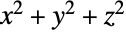
ContourPlot3D[x ^ 2 + y ^ 2 + z ^ 2 == 1, {x, -1, 1}, {y, -1, 1}, {z, -1, 1}]SliceContourPlot3D[x ^ 2 + y ^ 2 + z ^ 2, "CenterPlanes", {x, -1, 1}, {y, -1, 1}, {z, -1, 1}]テキスト
Wolfram Research (2015), SliceContourPlot3D, Wolfram言語関数, https://reference.wolfram.com/language/ref/SliceContourPlot3D.html (2022年に更新).
CMS
Wolfram Language. 2015. "SliceContourPlot3D." Wolfram Language & System Documentation Center. Wolfram Research. Last Modified 2022. https://reference.wolfram.com/language/ref/SliceContourPlot3D.html.
APA
Wolfram Language. (2015). SliceContourPlot3D. Wolfram Language & System Documentation Center. Retrieved from https://reference.wolfram.com/language/ref/SliceContourPlot3D.html