

ComplexPlot3D[f,{z,zmin,zmax}]
ComplexPlot3D
ComplexPlot3D[f,{z,zmin,zmax}]
詳細とオプション
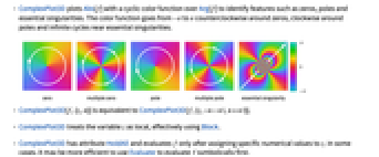
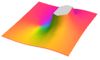
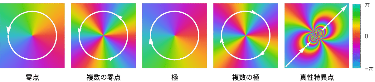
- ComplexPlot3Dは,Arg[f]上の循環的な色関数でAbs[f]をプロットして,零点,極,真性特異点等を識別する.色関数は
から
までで,零点の周りは反時計回り,極の周りは時計回りで,真性特異点の近くでは無限に循環する. - ComplexPlot3D[f,{z,n}]はComplexPlot3D[f,{z,-n-n I,n+n I}]に等しい.
- ComplexPlot3Dは,事実上Blockを使って,変数 z を局所的なものとして扱う.
- ComplexPlot3Dは属性HoldAllを有し,z に特定の数値を割り当てた後ではじめて f を評価する.場合によっては,Evaluateを使って最初に f を記号的に評価した方が効率がよいかもしれない.
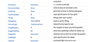
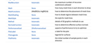
- ComplexPlot3DにはGraphics3Dと同じオプションに以下の追加・変更を加えたものが使える. [全オプションのリスト]
-
Axes True 軸を描くかどうか BoundaryStyle Black 曲面の境界線をどのように描くか BoxRatios {1,1,0.4`} 3D境界ボックスの割合 ClippingStyle Automatic 曲面の切り取られた部分をどのように描くか ColorFunction Automatic 曲面の色をどのように決定するか ColorFunctionScaling True ColorFunctionの引数をスケールするかどうか EvaluationMonitor None 関数評価のたびに評価する式 Exclusions Automatic 除外する x, y 曲線 ExclusionsStyle None 除外された曲線のところに何を描くか Filling None 各曲面の下の塗潰し FillingStyle Opacity[0.5`] 塗潰しに使うスタイル MaxRecursion Automatic 許容される再帰分割の最大数 Mesh None 各方向に何本のメッシュラインを描くか MeshFunctions {Abs[#2]&,Arg[#2]&} メッシュラインの置き方をどのように決めるか MeshShading None メッシュライン間の領域の陰影付けをどのように行うか MeshStyle Automatic メッシュラインのスタイル NormalsFunction Automatic 有効な曲面の法線をどのように決定するか PerformanceGoal $PerformanceGoal 最適化しようとするパフォーマンスの局面 PlotLegends None 曲面の凡例 PlotPoints Automatic 各方向のサンプル点の初期数 PlotRange {Full,Full,Automatic} 含める z あるいは他の値の範囲 PlotStyle Automatic 各曲面のスタイルのグラフィックス指示子 PlotTheme $PlotTheme プロットの全体的なテーマ RegionFunction (True&) 点を含めるかどうかの決定の仕方 ScalingFunctions None 個々の座標をどのようにスケールするか WorkingPrecision MachinePrecision 内部計算の精度 - ColorFunction->{cfunc,sfunc}は cfunc を使ってベースカラーを生成し,sfunc を使って特徴をハイライトする色を調整する.
- 次は,sfunc の可能な名前付き設定である.
-
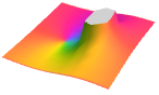
Automatic Abs[f]に基づいた自動陰影付け 
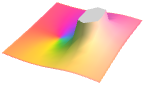
"MaxAbs" Abs[f]の大きい値の明るい陰影付け 
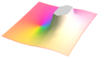
"LocalMaxAbs" Abs[f]の上側分位点の明るい陰影付け 

"GlobalAbs" Abs[f]の小さい値から大きい値への暗い陰影付けから明るい陰影付け 

"QuantileAbs" Abs[f]の分位数に基づいた暗い陰影付けから明るい陰影付け 
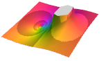
"CyclicLogAbs" Log[Abs[f]]の暗い陰影付けから明るい陰影付けの循環 
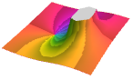
"CyclicArg" Arg[f]の暗い陰影付けから明るい陰影付けの循環 
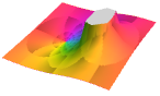
"CyclicLogAbsArg" Log[Abs[f]]とArg[f]の循環的陰影付け 
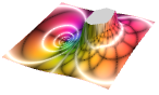
"CyclicReImLogAbs" Re[f]とIm[f]の暗い循環とLog[Abs[f]]の明るい循環 
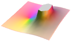
"ShiftedCyclicLogAbs" 閾値を超えた部分の Log[Abs[f]]の循環的陰影付け 
None 陰影は付けない - MeshFunctionsとRegionFunctionの中の関数に与えられる偏角は
と
である.ColorFunction内の関数には,デフォルトで,Re[z],Im[z],Abs[z],Arg[z],Re[f],Im[f],Abs[f],Arg[f]のスケールされたバージョンが渡される.
全オプションのリスト
例題
すべて開く すべて閉じる例 (3)
ComplexPlot3D[(z^2 + 1/z^2 - 1), {z, -2 - 2I, 2 + 2I}]ComplexPlot3D[(z^2 + 1/z^2 - 1), {z, -2 - 2I, 2 + 2I}, PlotLegends -> Automatic]ComplexPlot3D[(z^2 + 1/z^2 - 1), {z, -2 - 2I, 2 + 2I}, ColorFunction -> "CyclicLogAbsArg"]スコープ (22)
サンプリング (8)
ComplexPlot3D[((z + I)^3/(z + 1)^2)Exp[(1/z - 1 - I)], {z, -2 - 2I, 2 + 2I}]ComplexPlot3D[Exp[(5I/z)], {z, -1 - I, 1 + I}]ComplexPlot3D[Exp[-z] / z ^ 3, {z, Infinity}]デフォルトのメッシュは,一定のAbs[f]とArg[f]の曲線を示す:
ComplexPlot3D[z^3 - z^2 - 2, {z, -2 - 2I, 2 + 2I}, Mesh -> Automatic]極があるところでは,対数を使ってAbs[f]をスケールすると便利なことがよくある:
ComplexPlot3D[((z + 1 + I)/1 - I + I z - z^2), {z, -2 - 2I, 2 + 2I}, Mesh -> Automatic, ScalingFunctions -> "Log"]極があるところでは,対数を使ってAbs[f]のメッシュもスケールすると便利なことがよくある:
ComplexPlot3D[((z + 1 + I)/1 - I + I z - z^2), {z, -2 - 2I, 2 + 2I}, Mesh -> Automatic, MeshFunctions -> {Log[Abs[#2]]&, Arg[#2]&}]ComplexPlot3D[((z + 1 + I)/1 - I + I z - z^2), {z, -2 - 2I, 2 + 2I}, Mesh -> {Range[-1, 2, 0.1], Range[-Pi, Pi, Pi / 12]}, MeshFunctions -> {Log10[Abs[#2]]&, Arg[#2]&}, MeshStyle -> {Black, White}]メッシュに変更を加えてRe[f]とIm[f]の特定の値を示す:
ComplexPlot3D[(z^2 - I z - 1 + I/z - I), {z, -2 - 2I, 2 + 2I}, Mesh -> {Range[-4, 4, 0.5], Range[-2, 8, .5]}, MeshFunctions -> {Re[#2]&, Im[#2]&}]ComplexPlot3D[(z^2 - I z - 1 + I/z - I), {z, -2 - 2I, 2 + 2I}, ColorFunction -> "IslandColors", PlotLegends -> Automatic]プレゼンテーション (14)
ComplexPlot3D[(Sin[2π z]/z^3), {z, -2 - 2I, 2 + 2I}, PlotLegends -> Automatic]ComplexPlot3D[(z^2 + 1/z^2 - 1), {z, -2 - 2I, 2 + 2I}, Mesh -> 20, MeshFunctions -> {Log[Abs[#2]]&, Arg[#2]&}, MeshStyle -> {White, Black}]ComplexPlot3D[(z^2 + 1/z^2 - 1), {z, -2 - 2I, 2 + 2I}, ColorFunction -> "Rainbow", Exclusions -> None]ComplexPlot3D[(z^2 + 1/z^2 - 1), {z, -2 - 2I, 2 + 2I}, ScalingFunctions -> "Log"]ColorFunctionを変える:
ComplexPlot3D[(z^3 - 3/z), {z, -2 - 2I, 2 + 2I}, ColorFunction -> (Hue[#8 + 0.5]&)]"CyclicLogAbs"陰影付け関数を使って循環的に陰影を付けて一定のAbs[f]の等高線の外観を与える:
ComplexPlot3D[(z^4 - 1/z^2), {z, -2 - 2I, 2 + 2I}, ColorFunction -> "CyclicLogAbs", PlotLegends -> Automatic]"CyclicArg"陰影付け関数を使って循環的に陰影を付けて一定のArg[f]の等高線の外観を与える:
ComplexPlot3D[(z^4 - 1/z^2), {z, -2 - 2I, 2 + 2I}, ColorFunction -> "CyclicArg", PlotLegends -> Automatic]"CyclicLogAbsArg"陰影付け関数を使って循環的に陰影を付けて一定のAbs[f]とArg[f]の等高線の外観を与える:
ComplexPlot3D[(z^4 - 1/z^2), {z, -2 - 2I, 2 + 2I}, ColorFunction -> "CyclicLogAbsArg"]"GlobalAbs"陰影付け関数を使って零点(黒)と極(白)をハイライトする:
ComplexPlot3D[(z^4 - 1/z^2), {z, -2 - 2I, 2 + 2I}, ColorFunction -> "GlobalAbs", PlotLegends -> Automatic]"QuantileAbs"を使ってAbs[f]の小さい値を暗い色にし,Abs[f]の大きい値を明るい色にする:
ComplexPlot3D[(z^4 - 1/z^2), {z, -2 - 2I, 2 + 2I}, ColorFunction -> "QuantileAbs"]"MaxAbs"を使ってAbs[f]の大きい値を明るい色にする:
ComplexPlot3D[(z^4 - 1/z^2), {z, -2 - 2I, 2 + 2I}, ColorFunction -> "MaxAbs"]"LocalMaxAbs"を使ってAbs[f]の相対的に大きい値を明るい色にする:
ComplexPlot3D[(z^4 - 1/z^2), {z, -2 - 2I, 2 + 2I}, ColorFunction -> "LocalMaxAbs"]"CyclicReImLogAbs"を使って,Re[f]およびIm[f]に基づいて循環的に暗い色にし,Log[Abs[f]]に基づいて循環的に明るい色にする:
ComplexPlot3D[(z^3 - 1/z), {z, -2 - 2I, 2 + 2I}, ColorFunction -> "CyclicReImLogAbs"]"ShiftedCyclicLogAbs"を使って零点の周りに透明な色相環を生成し,Log[Abs[f]]に基づいて循環的な等高線を生成する:
ComplexPlot3D[(z^4 - 1/z^2), {z, -2 - 2I, 2 + 2I}, ColorFunction -> "ShiftedCyclicLogAbs"]オプション (95)
Axes (4)
デフォルトで,ComplexPlot3DにはAxesが使われる:
ComplexPlot3D[(z^2 + 1/z^2 - 1), {z, -2 - 2 I, 2 + 2 I}]ComplexPlot3D[(z^2 + 1/z^2 - 1), {z, -2 - 2 I, 2 + 2 I}, Axes -> False]AxesOriginを使って軸の交点を指定する:
ComplexPlot3D[(z^2 + 1/z^2 - 1), {z, -2 - 2 I, 2 + 2 I}, AxesOrigin -> {0, 0, 0}]{ComplexPlot3D[(z^2 + 1/z^2 - 1), {z, -2 - 2 I, 2 + 2 I}, Axes -> {True, False, False}], ComplexPlot3D[(z^2 + 1/z^2 - 1), {z, -2 - 2 I, 2 + 2 I}, Axes -> {False, True, False}], ComplexPlot3D[(z^2 + 1/z^2 - 1), {z, -2 - 2 I, 2 + 2 I}, Axes -> {False, False, True}]}AxesLabel (3)
ComplexPlot3D[(z^2 + 1/z^2 - 1), {z, -2 - 2 I, 2 + 2 I}, Axes -> True]ComplexPlot3D[(z^2 + 1/z^2 - 1), {z, -2 - 2 I, 2 + 2 I}, Axes -> True, AxesLabel -> z]ComplexPlot3D[(z^2 + 1/z^2 - 1), {z, -2 - 2 I, 2 + 2 I}, Axes -> True, AxesLabel -> {x, y, z}]AxesOrigin (2)
AxesStyle (4)
ComplexPlot3D[(z^2 + 1/z^2 - 1), {z, -2 - 2 I, 2 + 2 I}, AxesStyle -> Red]ComplexPlot3D[(z^2 + 1/z^2 - 1), {z, -2 - 2 I, 2 + 2 I}, AxesStyle -> {{Thick, Brown}, {Thick, Blue}, {Thick, Green}}]ComplexPlot3D[(z^2 + 1/z^2 - 1), {z, -2 - 2 I, 2 + 2 I}, Axes -> True, AxesStyle -> Green, TicksStyle -> Blue]ComplexPlot3D[(z^2 + 1/z^2 - 1), {z, -2 - 2 I, 2 + 2 I}, AxesStyle -> Green, LabelStyle -> Blue]BoundaryStyle (3)
ComplexPlot3D[(z + I/z - I), {z, -2 - 2I, 2 + 2I}]ComplexPlot3D[(z + I/z - I), {z, -2 - 2I, 2 + 2I}, BoundaryStyle -> Directive[StandardGray, Thick]]BoundaryStyleはRegionFunctionによって切り取られた穴には適用されるが,Exclusionsによって切り取られた穴には適用されない点に注意のこと:
ComplexPlot3D[(z + I/z - I), {z, -2 - 2I, 2 + 2I}, BoundaryStyle -> Directive[StandardGray, Thick], RegionFunction -> Function[{z, w}, Abs[z] ≥ 1 / 2]]BoxRatios (2)
AutomaticはPlotRangeからの自然なスケールを使う:
{ComplexPlot3D[Sin[z], {z, -2Pi - 2I, 2Pi + 2I}], ComplexPlot3D[Sin[z], {z, -2Pi - 2I, 2Pi + 2I}, BoxRatios -> Automatic]}BoxRatiosを使ってプロットの境界ボックスの相対的な次元を指定する:
ComplexPlot3D[(z^2 + 1/z^2 - 1), {z, -2 - 1I, 2 + I}, BoxRatios -> {2, 1, 2}]ClippingStyle (2)
ColorFunction (14)
ComplexPlot3D[(z^5 - 3/z^3), {z, -2 - 2I, 2 + 2I}, ColorFunction -> "GreenPinkTones", PlotLegends -> Automatic]LogGammaとLog[Gamma]は異なる分岐線を持つ:
{
ComplexPlot3D[LogGamma[z] , {z, -3 - 3I, 3 + 3I}, ColorFunction -> ColorData["CMYKColors"]],
ComplexPlot3D[Log[Gamma[z]] , {z, -3 - 3I, 3 + 3I}, ColorFunction -> ColorData["CMYKColors"]]
}カスタムのColorFunctionを指定する:
ComplexPlot3D[z^3 + 3z + 8 + (1/(z - 2)^2), {z, -3 - 3I, 3 + 3I}, ColorFunction -> (Hue[#8 + 0.5]&)]clrs = GrayLevel /@ Join[Range[0, 1, .25], Range[.75, 0, -.25]]ComplexPlot3D[z^3 + 3z + 8 + (1/(z - 2)^2), {z, -3 - 3I, 3 + 3I}, ColorFunction -> (Blend[clrs, #8]&)]色関数は8つの偏角(Re[z],Im[z],Abs[z],Arg[z],Re[f],Im[f],Abs[f],Arg[f])に依存する:
ComplexPlot3D[(z^2 + 1/z^2 - 1), {z, -2 - 2I, 2 + 2I}, ColorFunction -> {Hue[(#8/2π), 0.9^#7, If[#3 < 1.5, 1, 0.75]]&, None}, ColorFunctionScaling -> False, Exclusions -> None]ComplexPlot3D[(z^2 + 1/z^2 - 1), {z, -2 - 2I, 2 + 2I}, ColorFunction -> (Hue[#8, 1 - Cos[8π#8]^20, 1 - 0.2SawtoothWave[6#7]]&), ColorFunctionScaling -> False]ComplexPlot3D[z^3 - 2, {z, -2 - 2I, 2 + 2I}, ColorFunction -> (Hue[#7, 1 - 0.2SawtoothWave[8 #5], 1 - 0.2SawtoothWave[8#6]]&)]色関数に陰影を加えて,零点,極,鞍点等のグラフの特徴をハイライトすることができる."CyclicLogAbs"を使って循環的に陰影を付けて2のベキ乗における一定のAbs[f]の等高線の外観を与える:
ComplexPlot3D[(z^2 + 1/z^2 - 1), {z, -2 - 2I, 2 + 2I}, ColorFunction -> "CyclicLogAbs"]"CyclicArg"を使って循環的に陰影を付け,
/6の整数倍における一定のArg[f]の等高線の外観を与える:
ComplexPlot3D[(z^2 + 1/z^2 - 1), {z, -2 - 2I, 2 + 2I}, ColorFunction -> "CyclicArg"]"CylicLogAbsArg"陰影付け関数を使って"CyclicLogAbs"と"CyclicArg"の効果を組み合せる:
ComplexPlot3D[(z^2 + 1/z^2 - 1), {z, -2 - 2I, 2 + 2I}, ColorFunction -> "CyclicLogAbsArg"]陰影付けは任意のColorFunctionに適用できる:
ComplexPlot3D[(z^2 + 1/z^2 - 1), {z, -2 - 2I, 2 + 2I}, ColorFunction -> {"WatermelonColors", "CyclicLogAbsArg"}]"GlobalAbs"を使って零点(黒)と極(白)をハイライトする:
ComplexPlot3D[(z^2 + 1/z^2 - 1), {z, -2 - 2I, 2 + 2I}, ColorFunction -> "GlobalAbs"]"QuantileAbs"を使ってAbs[f]の相対的に大きい値における画像を明るくする:
ComplexPlot3D[(z^2 + 1/z^2 - 1), {z, -2 - 2I, 2 + 2I}, ColorFunction -> "QuantileAbs"]"MaxAbs"を使ってAbs[f]の大きい値における画像を明るくする:
ComplexPlot3D[(z^2 + 1/z^2 - 1), {z, -2 - 2I, 2 + 2I}, ColorFunction -> "MaxAbs"]"LocalMaxAbs"を使ってAbs[f]の相対的に大きい値における画像を明るくする:
ComplexPlot3D[(z^2 + 1/z^2 - 1), {z, -2 - 2I, 2 + 2I}, ColorFunction -> "LocalMaxAbs"]"ShiftedCyclicLogAbs"を使って,各零点の周りの色相環と,Log[Abs[f]]における循環的陰影付けを生成する:
ComplexPlot3D[(z^4 - 1/z^2), {z, -2 - 2I, 2 + 2I}, ColorFunction -> "ShiftedCyclicLogAbs"]"CyclicReImLogAbs"を使ってRe[f]とIm[f]におけるプロットを循環的に暗くし,Log[Abs[f]]におけるプロットを循環的に明るくする:
ComplexPlot3D[z^2 + 1, {z, -2 - 2I, 2 + 2I}, ColorFunction -> "CyclicReImLogAbs"]ColorFunctionScaling (1)
Exclusions (4)
ComplexPlot3D[z + Conjugate[z] Floor[Abs[z]], {z, -3 - 3I, 3 + 3I}]循環的色関数については,Abs[f]に基づく除外のみが表示される.しかし,非循環的な色関数については,Arg[f]に基づく除外も表示される:
ComplexPlot3D[z^4 - 1, {z, -2 - 2I, 2 + 2I}, ColorFunction -> "Rainbow", PlotLegends -> Automatic]ComplexPlot3D[z^2, {z, -3 - 3I, 3 + 3I}, Exclusions -> {Re[z] == 0}]ComplexPlot3D[((z + 2I)^2/(z + 2)^2), {z, -3 - 3I, 3 + 3I}, Exclusions -> {(Re[z] + 1)^2 + (Im[z] + 1)^2 == 2}]ComplexPlot3D[z + Conjugate[z] Floor[Abs[z]], {z, -3 - 3I, 3 + 3I}, Exclusions -> None]ExclusionStyle (1)
Filling (2)
ComplexPlot3D[(z^2 + 1/z^2 - 1), {z, -2 - 2I, 2 + 2I}, Filling -> Bottom]RegionFunctionで切り取られた領域に沿って塗潰しが行われる:
ComplexPlot3D[(z^2 + 1/z^2 - 1), {z, -2 - 2I, 2 + 2I}, Filling -> Bottom, RegionFunction -> (Abs[#1] ≤ 2&)]FillingStyle (3)
ComplexPlot3D[(z^2 + 1/z^2 - 1), {z, -2 - 2I, 2 + 2I}, Filling -> Bottom, FillingStyle -> Directive[Opacity[0.5], StandardGray]]平面Abs[f]=1まで,下からは赤で,上からは青で塗り潰す:
ComplexPlot3D[(z^2 + 1/z^2 - 1), {z, -2 - 2I, 2 + 2I}, Filling -> 1, FillingStyle -> {Red, Blue}]下からのみ平面Abs[f]=1まで塗り潰す:
ComplexPlot3D[(z^2 + 1/z^2 - 1), {z, -2 - 2I, 2 + 2I}, Filling -> 1, FillingStyle -> {Red, None}]ImageSize (7)
Tiny,Small,Medium,Largeのような名前付きのサイズを使う:
{ComplexPlot3D[(z^2 + 1/z^2 - 1), {z, -2 - 2I, 2 + 2I}, ImageSize -> Tiny], ComplexPlot3D[(z^2 + 1/z^2 - 1), {z, -2 - 2I, 2 + 2I}, ImageSize -> Small]}{ComplexPlot3D[(z^2 + 1/z^2 - 1), {z, -2 - 2I, 2 + 2I}, ImageSize -> 150], ComplexPlot3D[(z^2 + 1/z^2 - 1), {z, -2 - 2I, 2 + 2I}, AspectRatio -> 1.5, ImageSize -> 150]}{ComplexPlot3D[(z^2 + 1/z^2 - 1), {z, -2 - 2I, 2 + 2I}, ImageSize -> {Automatic, 150}], ComplexPlot3D[(z^2 + 1/z^2 - 1), {z, -2 - 2I, 2 + 2I}, AspectRatio -> 2, ImageSize -> {Automatic, 150}]}{ComplexPlot3D[(z^2 + 1/z^2 - 1), {z, -2 - 2I, 2 + 2I}, ImageSize -> UpTo[200]], ComplexPlot3D[(z^2 + 1/z^2 - 1), {z, -2 - 2I, 2 + 2I}, AspectRatio -> 2, ImageSize -> UpTo[200]]}グラフィックスの幅と高さを指定して,必要な場合はスペースで充填する:
ComplexPlot3D[(z^2 + 1/z^2 - 1), {z, -2 - 2I, 2 + 2I}, ImageSize -> {200, 200}, Background -> StandardGray]AspectRatioFullとすると使用可能なスペースが塗り潰される:
ComplexPlot3D[(z^2 + 1/z^2 - 1), {z, -2 - 2I, 2 + 2I}, AspectRatio -> Full, ImageSize -> {200, 200}, Background -> StandardGray]{ComplexPlot3D[(z^2 + 1/z^2 - 1), {z, -2 - 2I, 2 + 2I}, ImageSize -> {UpTo[150], UpTo[100]}], ComplexPlot3D[(z^2 + 1/z^2 - 1), {z, -2 - 2I, 2 + 2I}, AspectRatio -> 2, ImageSize -> {UpTo[150], UpTo[100]}]}ImageSizeFullを使ってオブジェクトの使用可能なスペースを塗り潰す:
Framed[Pane[ComplexPlot3D[(z^2 + 1/z^2 - 1), {z, -2 - 2I, 2 + 2I}, ImageSize -> Full, Background -> StandardGray], {200, 100}]]Framed[Pane[ComplexPlot3D[(z^2 + 1/z^2 - 1), {z, -2 - 2I, 2 + 2I}, AspectRatio -> Full, ImageSize -> {Scaled[0.5], Scaled[0.5]}, Background -> StandardGray], {200, 100}]]MaxRecursion (2)
領域関数が使われた場合,MaxRecursionは初期メッシュを適応させる:
Table[ComplexPlot3D[z / (z^2 + 1), {z, -2 - 2I, 2 + 2I}, PlotPoints -> 5, MaxRecursion -> mr, RegionFunction -> Function[{z}, Abs[z] ≤ 2], PlotLabel -> mr], {mr, 0, 2}]メッシュが使用される場合,MaxRecursionは初期メッシュを適応させる:
Table[ComplexPlot3D[z / (z^2 + 1), {z, -2 - 2I, 2 + 2I}, PlotPoints -> 8, MaxRecursion -> mr, Mesh -> 10, PlotLabel -> mr], {mr, 0, 2}]Mesh (2)
MeshFunctions (2)
MeshFunctionsを{Abs[f],Arg[f]}から{Re[f],Im[f]}に変更する:
ComplexPlot3D[z^2 + I, {z, -3 - 3I, 3 + 3I}, Mesh -> Automatic, MeshFunctions -> {Re[#2]&, Im[#2]&}]ComplexPlot3D[((z^2 + I)(z^2 + 2 + 2I)/(z + 2 + I)^2), {z, -3 - 3I, 3 + 3I}, Mesh -> 10, MeshFunctions -> {Log[Abs[#2]]&, Arg[#2]&}, PlotRange -> {0, 500}]MeshShading (2)
ComplexPlot3D[z^2 + 1, {z, -2 - 2I, 2 + 2I}, Mesh -> 20, MeshShading -> {{Automatic, Gray}, {Automatic, White}}]メッシュに陰影付けをしてAbs[f]をハイライトする:
ComplexPlot3D[(z - 1/z^2 + z + 1), {z, -2 - 2I, 2 + 2I}, Mesh -> 20, MeshShading -> {StandardGray, StandardBlue}, MeshFunctions -> {Log[Abs[#2]]&}]MeshStyle (2)
Abs[f]の方向に白いメッシュを,Arg[f]の方向に黒いメッシュを使う:
ComplexPlot3D[z^2 + 1, {z, -2 - 2I, 2 + 2I}, Mesh -> Automatic, MeshStyle -> {White, Black}]Abs[f]の方向に赤いメッシュを,Arg[f]の方向に青いメッシュを使う:
ComplexPlot3D[z^2 + 1, {z, -2 - 2I, 2 + 2I}, Mesh -> Automatic, MeshShading -> {{Gray, White}, {White, Gray}}, MeshStyle -> {Red, Blue}]NormalsFunction (2)
法線は自動的に計算される.Noneを使って多角形のすべてに平坦な陰影付けを行う:
ComplexPlot3D[1 / (z^2 + 1 - I), {z, -2 - 2I, 2 + 2I}, NormalsFunction -> None]ComplexPlot3D[1 / (z^2 + 1 - I), {z, -2 - 2I, 2 + 2I}, NormalsFunction -> ({Sin[2Pi#1], Cos[2Pi#2], 1}&)]PlotLegends (2)
Automaticの凡例は色と位相の関連を表示する.凡例のグレースケールの部分は色の陰影付けを示している:
ComplexPlot3D[Sin[z], {z, -π - 2I, π + 2I}, PlotLegends -> Automatic]ComplexPlot3D[Sin[z], {z, -π - 2I, π + 2I}, ColorFunction -> "CyclicLogAbs", PlotLegends -> Automatic]PlotPoints (2)
Table[ComplexPlot3D[(Sin[3z]/z^3), {z, -2 - 2I, 2 + 2I}, RegionFunction -> Function[{z}, Im[z^2] ≤ 1], PlotPoints -> i], {i, {5, 20}}]Table[ComplexPlot3D[(Sin[3z]/z^3), {z, -2 - 2I, 2 + 2I}, Mesh -> Automatic, PlotPoints -> i], {i, {5, 20}}]PlotRange (3)
Abs[f]の範囲を自動的に計算する:
ComplexPlot3D[(Sin[3z]/z^2), {z, -1 - I, 1 + I}]Abs[f]の範囲を指定する:
ComplexPlot3D[(Sin[3z]/z^2), {z, -1 - I, 1 + I}, PlotRange -> {0, 50}]f の定義域とAbs[f]の範囲の次元を指定する:
ComplexPlot3D[(Sin[3z]/z^2), {z, -1 - I, 1 + I}, PlotRange -> {{-2, 2}, {-2, 2}, {0, 50}}]PlotStyle (1)
PlotStyleを使って色を変更することができる:
ComplexPlot3D[(Sin[3z]/z^3), {z, -2 - 2I, 2 + 2I}, PlotStyle -> Opacity[0.5]]PlotTheme (1)
RegionFunction (3)
RegionFunctionを使って領域の形を適応させる:
ComplexPlot3D[(z^2 + 1/z^2 - 1), {z, -2 - 2I, 2 + 2I}, RegionFunction -> Function[{z}, Abs[z] ≤ 2]]RegionFunctionを使って零点と極を削除する:
ComplexPlot3D[(z^2 + 1/z^2 - 1), {z, -2 - 2I, 2 + 2I}, RegionFunction -> Function[{z, f}, 1 ≤ Abs[f] ≤ 2]]{ComplexPlot3D[(z^2 + 1/z^2 - 1), {z, -2 - 2I, 2 + 2I}, RegionFunction -> Function[{z, f}, -π / 2 ≤ Arg[z] < π]], ComplexPlot3D[(z^2 + 1/z^2 - 1), {z, -2 - 2I, 2 + 2I}, RegionFunction -> Function[{z, f}, -π / 2 ≤ Arg[f] < π]]}ScalingFunctions (8)
Abs[f]の方向に対数スケールを使う:
ComplexPlot3D[(z/z^2 - 1), {z, -2 - 2I, 2 + 2I}, ScalingFunctions -> "Log"]Abs[f]の方向に逆数軸スケールを使って,事実上零点と極を交換する:
ComplexPlot3D[(z/z^2 - 1), {z, -2 - 2I, 2 + 2I}, ScalingFunctions -> "Reciprocal"]スケーリング関数を組み合せて使う.Re[f]は反転させIm[f]はそのままにし,Abs[f]は逆数にする:
ComplexPlot3D[(z/z^2 - 1), {z, -2 - 2I, 2 + 2I}, ScalingFunctions -> {"Reverse", None, "Reciprocal"}]ComplexPlot3D[Exp[z] / (z - 5 - 5I) ^ 3, {z, 1 + I, 10 + 10I}, ScalingFunctions -> {"Log10", "Log10", "Log10"}]ComplexPlot3D[(z^2 + 1/z^2 - 1), {z, Infinity}]{ComplexPlot3D[(z^2 + 1/z^2 - 1), {z, Infinity}, ScalingFunctions -> {"Reverse", None, None}], ComplexPlot3D[(z^2 + 1/z^2 - 1), {z, Infinity}, ScalingFunctions -> {None, "Reverse", None}], ComplexPlot3D[(z^2 + 1/z^2 - 1), {z, Infinity}, ScalingFunctions -> {None, None, "Reverse"}]}ComplexPlot3D[(z^2 + 1/z^2 - 1), {z, Infinity}, ScalingFunctions -> {"Reciprocal", None, None}]Intervalを使って無限大領域の関心領域に焦点を当てる:
ComplexPlot3D[(z^2 + 1/z^2 - 1), {z, Infinity}, ScalingFunctions -> {{"Infinite", Interval[{-1, 1}]}, {"Infinite", Interval[{-1, 1}]}, {"Infinite", Interval[{-1, 1}]}}]Ticks (6)
ComplexPlot3D[z ^ 3 + 3 z + 8 + 1 / (z - 2) ^ 2, {z, -3 - 3 I, 3 + 3 I}]ComplexPlot3D[z ^ 3 + 3 z + 8 + 1 / (z - 2) ^ 2, {z, -3 - 3 I, 3 + 3 I}, Ticks -> None]ComplexPlot3D[z ^ 3 + 3 z + 8 + 1 / (z - 2) ^ 2, {z, -3 - 3 I, 3 + 3 I}, Ticks -> {{-2, 1, 2.5}, {-2, 1, 2}, {10, 20, 50}}]ComplexPlot3D[z ^ 3 + 3 z + 8 + 1 / (z - 2) ^ 2, {z, -3 - 3 I, 3 + 3 I}, Ticks -> {{{-2, -a}, {1, b}, {2.5, c}}, {{-2, -a}, {1, b}, {2, a}}, {{10, f}, {30, g}, {50, h}}}]ComplexPlot3D[z ^ 3 + 3 z + 8 + 1 / (z - 2) ^ 2, {z, -3 - 3 I, 3 + 3 I}, Ticks -> {{{-2, -a, .1}, {1, b, .07}, {2.2, c, .24}}, {{-2, -a, .15}, {1, b, .06}, {2, a, .06}}, {{10, f, .01}, {30, g, .22}, {50, h, .12}}}]ComplexPlot3D[z ^ 3 + 3 z + 8 + 1 / (z - 2) ^ 2, {z, -3 - 3 I, 3 + 3 I}, Ticks -> {{{-2, -a, .1, Directive[Thick, Blue]}, {1, b, .07, Directive[Thick, Blue]}, {2.2, c, .24, Directive[Thick, Blue]}}, {{-2, -a, .15, Directive[Blue]}, {1, b, .06, Directive[Blue]}, {2, a, .06, Directive[Blue]}}, {{10, f, .01, Directive[Thick, Red]}, {30, g, .22, Directive[Thick, Red]}, {50, h, .12, Directive[Thick, Red]}}}]TicksStyle (3)
デフォルトで,目盛と目盛ラベルには軸と同じスタイルが使われる:
ComplexPlot3D[z ^ 3 + 3 z + 8 + 1 / (z - 2) ^ 2, {z, -3 - 3 I, 3 + 3 I}, AxesStyle -> Directive[Red, Thick]]ComplexPlot3D[z ^ 3 + 3 z + 8 + 1 / (z - 2) ^ 2, {z, -3 - 3 I, 3 + 3 I}, TicksStyle -> Directive[Blue, 12]]ComplexPlot3D[z ^ 3 + 3 z + 8 + 1 / (z - 2) ^ 2, {z, -3 - 3 I, 3 + 3 I}, TicksStyle -> {Directive[Green, 12], Directive[Blue, 12], Directive[Red, 12]}]アプリケーション (26)
基本的なアプリケーション (10)
複素関数
について,Abs[f]を複素平面上でプロットする.曲面上の点は(デフォルトで)Arg[f]によって彩色され,その情報が任意の凡例に記録される.
ComplexPlot3D[z, {z, -2 - 2I, 2 + 2I}, PlotLegends -> Automatic]ComplexPlot3D[z^3, {z, -2 - 2I, 2 + 2I}, PlotLegends -> Automatic]ComplexPlot3D[1 / z, {z, -2 - 2I, 2 + 2I}, PlotLegends -> Automatic]ComplexPlot3D[Exp[I / z], {z, -0.5 - 0.5I, 0.5 + 0.5I}]PlotRangeを使って極の近くのグラフの高さを制御する:
ComplexPlot3D[Exp[I / z], {z, -0.5 - 0.5I, 0.5 + 0.5I}, PlotRange -> {0, 10^6}]極がある関数に対数スケール関数を使うと,より視覚的に魅力的なプロットが生成されるかもしれない:
ComplexPlot3D[Exp[I / z], {z, -0.5 - 0.5I, 0.5 + 0.5I}, ScalingFunctions -> "Log"]ScalingFunctions"Reciprocal"を使うと,事実上,高さについて零点と極が入れ替えられるが,色は変化しない:
{ComplexPlot3D[((z - 1)^2/z + 1), {z, -2 - 2I, 2 + 2I}, ScalingFunctions -> None],
ComplexPlot3D[((z - 1)^2/z + 1), {z, -2 - 2I, 2 + 2I}, ScalingFunctions -> "Reciprocal"]}
の鞍点
で
かつ
."CyclicLogAbs"を使って2のベキ乗で生起する鞍点をハイライトする:
ComplexPlot3D[z^3 + 1, {z, -2 - 2I, 2 + 2I}, ColorFunction -> "CyclicLogAbs"]ComplexPlot3D[z^3 + 1, {z, -2 - 2I, 2 + 2I}, Mesh -> {Range[0, 5], Range[-Pi, Pi, Pi / 4]}, MeshFunctions -> {Log[Abs[#2]]&, Arg[#2]&}, PlotPoints -> 75]次のプロットはJoukowski変換の複数の特徴を示している.
に単純零点があるが,これはグラフの高さとこれらの点に色が収束しているという事実,また,これらの点の周りで(凡例とも一致して)色が反時計回りに青から緑さらに赤へと循環していることから明白である.同様に,
に,高さが無限で色は収束するが時計回りに循環する単純極がある.また,
には鞍点があり,赤と青の境界に分岐線がある:
ComplexPlot3D[z + (1/z), {z, -2 - 2I, 2 + 2I}, ColorFunction -> "DarkRainbow", PlotLegends -> Automatic]次のプロットは,
に単純零点,
に二重極,
に鞍点がある関数を示している:
ComplexPlot3D[(10(z^2 + 2z + 2)/(z - 1)^2), {z, -2 - 2I, 2 + 2I}, ColorFunction -> "CyclicLogAbs", ScalingFunctions -> "Log"]その他のアプリケーション (16)
古典的 (2)
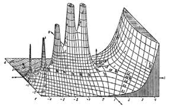
JanhkeとEmdeによる有名な複素プロット (Tables of Functions with Formulas and Curves, 4th ed., Dover, 1945)を再生する:
ComplexPlot3D[Gamma[z], {z, -4.5 - 2.5I, 4.5 + 2.5I}, Filling -> Bottom, PlotRange -> {0, 6}, PlotPoints -> 50, Exclusions -> None, Mesh -> {Join[10 ^ Range[-4, 0, 0.5], Range[0, 6, 0.5]], Range[-Pi, Pi, Pi / 6]}, ViewPoint -> {-.8, -3, 1}, Boxed -> False, AxesOrigin -> {0, 0, 0}, AxesLabel -> {"x", "y", "z"}]JanhkeとEmdeによる有名な複素プロット(Eugene Jahnke and Fritz Emde, Tables of Functions with Formulas and Curves, 4th ed., Dover, 1945)の3D版を作成する:
ComplexPlot3D[BesselJ[0, z] + I BesselY[0, z], {z, -4 - 1.5I, 2 + 1.5I}, Mesh -> Automatic, PlotRange -> {0, 4}, BoxRatios -> {2, 1, (4/3)}, ViewPoint -> Above]一般 (6)
ComplexPlot3D[Cos[z], {z, -2Pi - 3I, 2Pi + 3I}, ColorFunction -> "CyclicLogAbsArg", ScalingFunctions -> "Log"]複素変数の複素関数の特徴を可視化する.次のプロットは,
に三重零点,
に単純零点,
に単純極,
に二重極があることを示している:
ComplexPlot3D[((z + 1 + I)^3(z^2 + 1)Exp[3 / z]/(z - 1)^2(z + 1)), {z, -2 - 2I, 2 + 2I}, PlotRange -> {0, 10^4}]Manipulate[ComplexPlot3D[z^n - 1, {z, -2 - 2 I, 2 + 2 I}, ScalingFunctions -> "Log"], {n, 2, 20, 1}]ComplexPlot3D[ChebyshevT[5, z], {z, -1.5 - 1.5 I, 1.5 + 1.5 I}, ColorFunction -> "CyclicLogAbs", ScalingFunctions -> "Log", ViewPoint -> {1, -2.4, 0.8}]幾何級数の部分和のプロットは,無限級数が
で発散することを示唆している:
Manipulate[ComplexPlot3D[Sum[z^k, {k, 0, kmax}], {z, -2 - 2 I, 2 + 2 I}, ColorFunction -> "CyclicLogAbs", ScalingFunctions -> "Log"], {{kmax, 10, "max k"}, 1, 35, 1}]ComplexPlot3D[(z - 2 + 2I/-3 + 3I - z), {z, -5 - 5 I, 5 + 5 I}, PlotPoints -> 50, Mesh -> 20, MeshStyle -> {Directive[Thick, White], Black}, MeshFunctions -> {Log[Abs[#2]]&, Arg[#2]&}, Exclusions -> None]特殊関数 (2)
ComplexPlot3D[Erf[z], {z, -5 - 5 I, 5 + 5 I}, ScalingFunctions -> "Log10"]ComplexPlot3D[(Gamma[z - I]^2/Gamma[z + I]^2), {z, -5.5 - 2I, 2 + 2I}, ColorFunction -> "ShiftedCyclicLogAbs", ScalingFunctions -> "Log"]Re[z]>0についてはLog[z2]2Log[z]だがRe[z]≤0についてはそうではないことを視覚的に思い出させるもの:
{ComplexPlot3D[Log[z^2], {z, -2 - 2I, 2 + 2I}], ComplexPlot3D[2Log[z], {z, -2 - 2I, 2 + 2I}]}解析関数 (2)
ComplexPlot3D[Sin[z / 2], {z, -4 - 4I, 4 + 4I}, Mesh -> 20, MeshFunctions -> {Re[#2]&, Im[#2]&}, MeshShading -> {{White, StandardGray}, {StandardGray, White}}]{ComplexPlot3D[(z^2 + 1/z^2 - 1), {z, -2 - 2I, 2 + 2I}, ColorFunction -> "CyclicLogAbsArg"],
ComplexPlot3D[(z^2 + 1/Conjugate[z]^2 - 1), {z, -2 - 2I, 2 + 2I}, ColorFunction -> "CyclicLogAbsArg"]}物理 (2)
における,値は等しいが反対の電荷を持つ2つの点電荷についての力線(黒)とポテンシャル線(白)をプロットする:
ComplexPlot3D[(z + 1/z - 1), {z, -3 - 3I, 3 + 3I}, Exclusions -> None, PlotPoints -> 40, Mesh -> 30, MeshFunctions -> {Log10[Abs[#2]]&, Arg[#2]&}, MeshStyle -> {White, Black}, ColorFunction -> "GlobalAbs", ViewPoint -> {0, 0, 2}]複雑な流体速度ポテンシャルを,外部からコーナーへの流れについての対応する流線でプロットする:
ComplexPlot3D[(-I z)^2 / 3 - (-z)^2 / 3, {z, -3 - 3I, 3 + 3I}, Mesh -> {Range[0, 3, .2]}, MeshFunctions -> {Im[#2]&}, RegionFunction -> Function[{z}, Arg[z] < -π / 2 || Arg[z] > 0], BoundaryStyle -> None]変換 (2)
ft = FourierTransform[Exp[-x^2]UnitStep[x], x, ω]ComplexPlot3D[Evaluate[ft], {ω, -10 - 10I, 10 + 0I}, ScalingFunctions -> "Log"]lt = LaplaceTransform[t^2 SawtoothWave[t / 2], t, s]//ApartComplexPlot3D[Evaluate[lt], {s, -10 - 15I, 20 + 15I}, ScalingFunctions -> "Log"]特性と関係 (8)
ComplexPlot3DはPlot3Dの特殊ケースである:
{ComplexPlot3D[Log[z], {z, -3 - 3I, 3 + 3I}], Plot3D[Abs[Log[x + I * y]], {x, -3, 3}, {y, -3, 3}]}ComplexPlotは関数の引数と大きさを色で示す:
ComplexPlot[Log[z], {z, 3}]複素数の配列にComplexArrayPlotを使う:
ComplexArrayPlot[Table[x ^ 3 + I y ^ 2, {x, -2, 2, 0.1}, {y, -2, 2, 0.1}]]ReImPlotとAbsArgPlotを使って複素数値を実数上にプロットする:
ReImPlot[Log[x], {x, -3, 3}]AbsArgPlot[Log[x], {x, -3, 3}]ComplexListPlotを使って平面上に複素数値の位置を示す:
ComplexListPlot[RandomComplex[{-3 - 3I, 3 + 3I}, 100]]ComplexContourPlotは複素数値の上に曲線をプロットする:
ComplexContourPlot[Abs[Log[z]] == 1, {z, 3}]ComplexRegionPlotは複素数値の上に領域をプロットする:
ComplexRegionPlot[Abs[Log[z]] < 1, {z, 3}]ComplexStreamPlotとComplexVectorPlotは複素数を方向として扱う:
ComplexStreamPlot[Log[z], {z, 3}]ComplexVectorPlot[Log[z], {z, 3}]テキスト
Wolfram Research (2019), ComplexPlot3D, Wolfram言語関数, https://reference.wolfram.com/language/ref/ComplexPlot3D.html (2021年に更新).
CMS
Wolfram Language. 2019. "ComplexPlot3D." Wolfram Language & System Documentation Center. Wolfram Research. Last Modified 2021. https://reference.wolfram.com/language/ref/ComplexPlot3D.html.
APA
Wolfram Language. (2019). ComplexPlot3D. Wolfram Language & System Documentation Center. Retrieved from https://reference.wolfram.com/language/ref/ComplexPlot3D.html
BibTeX
@misc{reference.wolfram_2026_complexplot3d, author="Wolfram Research", title="{ComplexPlot3D}", year="2021", howpublished="\url{https://reference.wolfram.com/language/ref/ComplexPlot3D.html}", note=[Accessed: 10-September-2026]}
BibLaTeX
@online{reference.wolfram_2026_complexplot3d, organization={Wolfram Research}, title={ComplexPlot3D}, year={2021}, url={https://reference.wolfram.com/language/ref/ComplexPlot3D.html}, note=[Accessed: 10-September-2026]}