ComplexRegionPlot[pred,{z,zmin,zmax}]
绘制复平面上 pred 为 True 的区域.
ComplexRegionPlot[{pred1,pred2,…},{z,zmin,zmax}]
绘制由多个谓词 predi 给定的区域.
ComplexRegionPlot
ComplexRegionPlot[pred,{z,zmin,zmax}]
绘制复平面上 pred 为 True 的区域.
ComplexRegionPlot[{pred1,pred2,…},{z,zmin,zmax}]
绘制由多个谓词 predi 给定的区域.
更多信息和选项
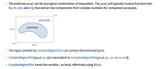
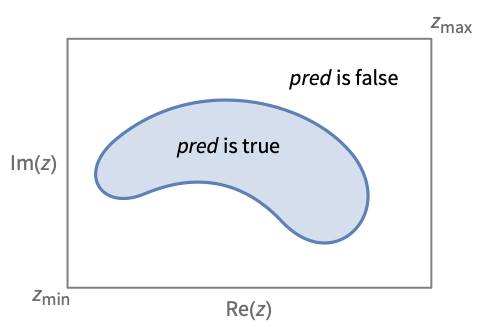
- 谓词 predi 可为为任意不等式的逻辑组合. predi 通常会涉及如 Re、Im、Abs 和 Arg 这样的函数,从复数中提取实数以进行比较.
- ComplexRegionPlot 绘制的区域可包含不相连的部分.
- ComplexRegionPlot[pred,{z,n}] 等价于 ComplexRegionPlot[pred,{z,-n-n I,n+n I}].
- ComplexRegionPlot 将变量 z 视为局部变量,相当于使用 Block.
- ComplexRegionPlot 具有属性 HoldAll,只在对 z 赋值后才计算 pred. 某些情况下,先用 Evaluate 对 pred 进行符号式计算效率更高.
- 以下封装 w 可用于 predi:
-
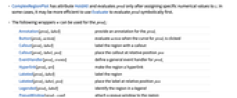
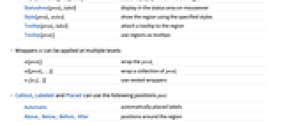
Annotation[predi,label] 为 predi 提供注释 Button[predi,action] 当 predi 的曲线被点击时执行 action Callout[predi,label] 用标注 (callout) 标记区域 Callout[predi,label,pos] 将标注放置在相对位置 pos EventHandler[predi,events] 定义 predi 的通用事件处理程序 Hyperlink[predi,uri] 把区域变为一个超链接 Labeled[predi,label] 标记区域 Labeled[predi,label,pos] 将标签放置在相对位置 pos Legended[predi,label] 在图例中标识区域 PopupWindow[predi,cont] 为区域添加弹出窗口 StatusArea[predi,label] 当鼠标移过时在状态栏中显示 Style[predi,styles] 用指定样式显示区域 Tooltip[predi,label] 为区域添加提示条 Tooltip[predi] 将区域用作提示条 - 可在多个层级上应用封装 w:
-
w[predi] 封装 predi w[{predi,…}] 封装一组 predi w1[w2[…]] 使用嵌套封装 - Callout、Labeled 和 Placed 可使用以下位置 pos:
-
Automatic 自动放置标签 Above, Below, Before, After 区域周围的位置 z z 附近的位置 {pos,epos} 在区域的相对位置 pos 处放置的标签中的 epos - ComplexRegionPlot 和 Graphics 有相同的选项,不同之处和更多选项如下所示: [所有选项的列表]
-
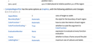
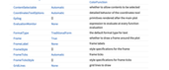
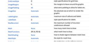
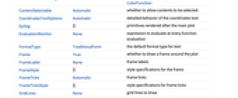
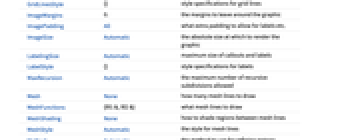
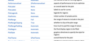
AspectRatio 1 高宽比 BoundaryStyle Automatic 每个区域的边界的样式 ColorFunction Automatic 怎样为每个区域的内部着色 ColorFunctionScaling True 是否对 ColorFunction 的参数进行缩放 EvaluationMonitor None 每次运行函数时要计算的表达式 Frame True 是否为图形绘制边框 LabelingSize Automatic 最大化标注和标签的大小 MaxRecursion Automatic 递归子划分的最大数量 Mesh None 绘制多少条网格线 MeshFunctions {#1&,#2&} 绘制什么样的网格线 MeshShading None 怎样处理网格线之间区域的色调 MeshStyle Automatic 网格线的样式 Method Automatic 细化区域所用的方法 PerformanceGoal $PerformanceGoal 优化的目标 PlotLabels None 曲线的标签 PlotLegends None 区域的图例 PlotPoints Automatic 初始采样点的个数 PlotRange Full 绘图中要包含的值的范围 PlotRangeClipping True 在绘图范围边界处是否进行剪切 PlotRangePadding Automatic 对值的范围进行多少填充 PlotStyle Automatic 指定区域的样式的图形指令 PlotTheme $PlotTheme 绘图的整体外观主题 TextureCoordinateFunction Automatic 怎样确定纹理的坐标 TextureCoordinateScaling True 是否对 TextureCoordinateFunction 的参数进行缩放 WorkingPrecision MachinePrecision 内部计算使用的精度 - PlotLegends 的常见设置有:
-
None 没有图例 Automatic 自动确定图例 "Expressions" 用 f1、f2、… 作为图例标签 {lbl1,lbl2,…} 用 lbl1、lbl2、… 作为图例标签 Placed[lspec,…] 指定图例的放置 - PlotStylesty 指定每组数据使用的样式. 可能的设置包括:
-
{sty1,sty2,…} 针对各个数据集的一系列样式 <|"key"val,…|> 针对不同层级的数据的样式元素 - 接受的键有:
-
"Base" 所有 fi 的整体样式 "Functions" 针对每个 fi 的样式列表 styi - ColorData["DefaultPlotColors"] 给出 PlotStyle 使用的默认颜色序列.
- ComplexRegionPlot 首先在由 PlotPoints 指定的等间隔采样点组成的网格上计算 pred. 然后使用一种自适应算法进行至多 MaxRecursion 次子划分,试图找出所有 pred 为 True 的区域的边界.
- 应该认识到由于使用的采样点数量有限,ComplexRegionPlot 可能会丢失某些 pred 为 True 的区域. 为确保结果正确,可以尝试增大 PlotPoints 和 MaxRecursion 的设置.
- 采用默认设置 PlotRange->Full 时,ComplexRegionPlot 将明确包含 z 从 zmin 到 zmax 内的所有值.
- ComplexRegionPlot 通常只能找到值为真的区域;找不到仅为线或点的区域.
- 为 MeshFunctions 中的函数提供的参数为 z. 默认情况下,为 ColorFunction 和 TextureCoordinateFunction 提供的是 Re[z]、Im[z]、Abs[z]、Arg[z] 经过缩放的值.
所有选项的列表
范例
打开所有单元 关闭所有单元基本范例 (5)
ComplexRegionPlot[Abs[z] ≤ 1, {z, -1 - I, 1 + I}]ComplexRegionPlot[Abs[z] ≤ 1, {z, 1}]ComplexRegionPlot[0 < Arg[z] < 2π / 3, {z, 5}]ComplexRegionPlot[{Re[z ^ 2] < 1, Im[z ^ 2] < 1}, {z, 2}]ComplexRegionPlot[Abs[z] ≤ 1 && Abs[Arg[z]] > π / 4, {z, -1 - I, 1 + I}, PlotStyle -> Yellow]范围 (23)
采样 (3)
ComplexRegionPlot[Abs[Nest[(# ^ 2 + z)&, z, 8]] < 2, {z, -2 - 1.5I, 1 + 1.5I}, Mesh -> All]用 PlotPoints 和 MaxRecursion 控制自适应采样:
Table[ComplexRegionPlot[1 < Abs[Sin[2 z] Cosh[2 z]] < 4, {z, -2 - 2I, 2 + 2I}, PlotPoints -> pp, MaxRecursion -> mr, Mesh -> None], {mr, {0, 2}}, {pp, {5, 15}}]ComplexRegionPlot[Re[z^2] ≤ 2 && Im[z^2] > 1, {z, -3 - 3I, 3 + 3I}]添加标签和图例 (9)
用 Labeled 标记区域:
ComplexRegionPlot[Labeled[Abs[z] < 1, "disk", Above], {z, -1.5 - 1.5I, 1.5 + 1.5I}]ComplexRegionPlot[{Labeled[Abs[z] < 1, "disk", Right], Labeled[Re[z] < 1, "rectangle", Below]}, {z, -1.5 - 1.5I, 1.5 + 1.5I}]Table[ComplexRegionPlot[Labeled[Abs[z] < 1, "disk", pos], {z, -1.5 - 1.5I, 1.5 + 1.5I}, PlotLabel -> pos], {pos, {Top, Bottom, Left, Right}}]用 Callout 标记区域:
ComplexRegionPlot[Callout[1 < Abs[Sin[2 z] Sinh[2 z]] < 6, "region", {1, 1}], {z, -2 - 2I, 2 + 2I}]ComplexRegionPlot[{Callout[1 < Abs[Sin[2 z] Sinh[2 z]] < 6, "region", {1, 1}], Callout[Abs[z] < 2, "disk", {1, -1}]}, {z, -2 - 2I, 2 + 2I}]ComplexRegionPlot[Callout[Abs[Sin[2 z] Sinh[2 z]] < 6, "region", {0, 0}], {z, -2 - 2I, 2 + 2I}]用 PlotLegends 添加图例:
ComplexRegionPlot[{1 < Abs[Sin[2 z] Sinh[2 z]] < 6, Abs[z] < 2}, {z, -2 - 2I, 2 + 2I}, PlotLegends -> "Expressions"]ComplexRegionPlot[{1 < Abs[Sin[2 z] Sinh[2 z]] < 6, Abs[z] < 2}, {z, -2 - 2I, 2 + 2I}, PlotLegends -> Automatic]用 Legended 添加图例:
ComplexRegionPlot[{Legended[1 < Abs[Sin[2 z] Sinh[2 z]] < 6, "region"], Legended[Abs[z] < 2, "disk"]}, {z, -2 - 2I, 2 + 2I}]演示 (11)
为区域设置明确的 PlotStyle:
ComplexRegionPlot[Abs[z] ≤ 1 && Abs[Arg[z]] > π / 4, {z, -1 - I, 1 + I}, PlotStyle -> Yellow]为区域的边界设置明确的 BoundaryStyle:
ComplexRegionPlot[Abs[z] ≤ 1 && Abs[Arg[z]] > π / 4, {z, -1 - I, 1 + I}, PlotStyle -> Yellow, BoundaryStyle -> Dashed]ComplexRegionPlot[{3 ≤ Abs[z] ≤ 4, Abs[z] < 2}, {z, -4 - 4I, 4 + 4I}, FrameLabel -> {"real", "imaginary"}, PlotLabel -> "shapes", PlotLabels -> {"annulus", "disk"}]ComplexRegionPlot[{Callout[3 ≤ Abs[z] ≤ 4, "annulus"], Labeled[Abs[z] < 2, "disk", Below]}, {z, -4 - 4I, 4 + 4I}]ComplexRegionPlot[{3 ≤ Abs[z] ≤ 4, Abs[z] < 2}, {z, -4 - 4I, 4 + 4I}, PlotLegends -> "Expressions"]ComplexRegionPlot[{3 ≤ Abs[z] ≤ 4, Abs[z] < 2}, {z, -4 - 4I, 4 + 4I}, PlotLegends -> Automatic]ComplexRegionPlot[2 ≤ Abs[z] ≤ 4, {z, -4 - 4I, 4 + 4I}, ColorFunction -> Hue, PlotLegends -> Automatic]ComplexRegionPlot[2 ≤ Abs[z] ≤ 4, {z, -4 - 4I, 4 + 4I}, Mesh -> 8, MeshStyle -> Directive[Red, Dashed]]ComplexRegionPlot[2 ≤ Abs[z] ≤ 4, {z, -4 - 4I, 4 + 4I}, Mesh -> 8, MeshShading -> {{Yellow, Orange}, {Pink, Red}}]ComplexRegionPlot[Abs[Nest[(# ^ 2 + z)&, z, 8]] < 2, {z, -2 - 1.5I, 1 + 1.5I}, ColorFunction -> Function[{re, im, abs, arg}, Hue[Nest[(# ^ 2 + re)&, re, 8]]], ColorFunctionScaling -> False, PlotPoints -> 50]ComplexRegionPlot[2 ≤ Abs[z] ≤ 4, {z, -4 - 4I, 4 + 4I}, PlotTheme -> "Scientific"]选项 (59)
BoundaryStyle (4)
ComplexRegionPlot[Abs[z^4 - z / 5 + 1] ≤ 1, {z, -1 - I, 1 + I}]用 None 显示没有边界的区域:
ComplexRegionPlot[Abs[z^4 - z / 5 + 1] ≤ 1, {z, -1 - I, 1 + I}, BoundaryStyle -> None]ComplexRegionPlot[Abs[z^4 - z / 5 + 1] ≤ 1, {z, -1 - I, 1 + I}, BoundaryStyle -> Red]ComplexRegionPlot[Abs[z^4 - z / 5 + 1] ≤ 1, {z, -1 - I, 1 + I}, BoundaryStyle -> Directive[Thickness[Medium], Dashed]]ColorFunction (5)
用缩放过的 Re[z]、Im[z]、Abs[z] 或 Arg[z] 为区域着色:
{
ComplexRegionPlot[Abs[z] < 2, {z, -2 - 2I, 2 + 2I}, ColorFunction -> (Hue[#1]&)],
ComplexRegionPlot[Abs[z] < 2, {z, -2 - 2I, 2 + 2I}, ColorFunction -> (Hue[#2]&)],
ComplexRegionPlot[Abs[z] < 2, {z, -2 - 2I, 2 + 2I}, ColorFunction -> (Hue[#3]&)],
ComplexRegionPlot[Abs[z] < 2, {z, -2 - 2I, 2 + 2I}, ColorFunction -> (Hue[#4]&)]
}已命名颜色函数沿缩放过的 Arg[z] 方向进行着色:
ComplexRegionPlot[Abs[z] < 1, {z, -1 - I, 1 + I}, ColorFunction -> "Rainbow"]ComplexRegionPlot[Abs[z^4 - z / 5 + 1] ≤ 1, {z, -1 - I, 1 + I}, ColorFunction -> Function[{z}, ColorData["SolarColors"][Abs[z]]], ColorFunctionScaling -> False]ColorFunction 比 PlotStyle 的优先级高:
ComplexRegionPlot[Abs[z^4 - z / 5 + 1] ≤ 1, {z, -1 - I, 1 + I}, ColorFunction -> "DarkRainbow", PlotStyle -> Directive[Opacity[0.5], Red]]ColorFunction 比 MeshShading 的优先级低:
ComplexRegionPlot[Abs[z^4 - z / 5 + 1] ≤ 1, {z, -1 - I, 1 + I}, Mesh -> 30, MeshShading -> {{Gray, Automatic}, {Automatic, Gray}}, ColorFunction -> "DarkRainbow"]ColorFunctionScaling (1)
用未经缩放的 Re[z]、Im[z]、Abs[z] 或 Arg[z] 为区域着色:
{
ComplexRegionPlot[Abs[z] < 2, {z, -2 - 2I, 2 + 2I}, ColorFunction -> (Hue[#1]&), ColorFunctionScaling -> False],
ComplexRegionPlot[Abs[z] < 2, {z, -2 - 2I, 2 + 2I}, ColorFunction -> (Hue[#2]&), ColorFunctionScaling -> False],
ComplexRegionPlot[Abs[z] < 2, {z, -2 - 2I, 2 + 2I}, ColorFunction -> (Hue[#3]&), ColorFunctionScaling -> False],
ComplexRegionPlot[Abs[z] < 2, {z, -2 - 2I, 2 + 2I}, ColorFunction -> (Hue[#4]&), ColorFunctionScaling -> False]
}LabelingSize (2)
ComplexRegionPlot[Callout[Abs[z] ≤ 1 && Abs[Arg[z]] > π / 4, "region"], {z, -1 - I, 1 + I}, PlotStyle -> Yellow]ComplexRegionPlot[Callout[Abs[z] ≤ 1 && Abs[Arg[z]] > π / 4, "region"], {z, -1 - I, 1 + I}, PlotStyle -> Yellow, LabelingSize -> 25]MaxRecursion (1)
Mesh (7)
ComplexRegionPlot[Abs[z] ≤ 1, {z, -1 - I, 1 + I}]{ComplexRegionPlot[Abs[z] ≤ 1, {z, -1 - I, 1 + I}, Mesh -> Full],
ComplexRegionPlot[Abs[z] ≤ 1, {z, -1 - I, 1 + I}, Mesh -> All]}ComplexRegionPlot[Abs[z] ≤ 1, {z, -1 - I, 1 + I}, Mesh -> 10]在 Re[z] 方向上显示 3 条网格线,在 Im[z] 方向上显示 6 条网格线:
ComplexRegionPlot[Abs[z] ≤ 1, {z, -1 - I, 1 + I}, Mesh -> {3, 6}]ComplexRegionPlot[Abs[z] ≤ 1, {z, -1 - I, 1 + I}, Mesh -> {{-1 / 2, 1 / 2}, {0}}]ComplexRegionPlot[Abs[z] ≤ 1, {z, -1 - I, 1 + I}, Mesh -> {{{-1 / 2, Red}, {1 / 2, Red}}, {{0, Dashed}}}]ComplexRegionPlot[Abs[z] > 1 && Pi / 4 < Abs[Arg[z]] < 3Pi / 4, {z, -2 - 2I, 2 + 2I}, Mesh -> 10]MeshFunctions (2)
{ComplexRegionPlot[Abs[z] ≤ 1, {z, -1 - I, 1 + I}, Mesh -> 10, MeshFunctions -> {Re[#]&}], ComplexRegionPlot[Abs[z] ≤ 1, {z, -1 - I, 1 + I}, Mesh -> 10, MeshFunctions -> {Im[#]&}]}ComplexRegionPlot[Abs[z] ≤ 1, {z, -1 - I, 1 + I}, Mesh -> 10, MeshFunctions -> {Abs[#]&}]MeshShading (4)
用 None 移除区域:
ComplexRegionPlot[Abs[z] ≤ 1, {z, -1 - I, 1 + I}, Mesh -> 8, MeshFunctions -> {Re[#] - Im[#]&}, MeshShading -> {Red, None}]ComplexRegionPlot[Abs[z] ≤ 1, {z, -1 - I, 1 + I}, Mesh -> 10, MeshShading -> {{Red, Yellow}, {Pink, Orange}}]MeshShading 比 PlotStyle 的优先级高:
ComplexRegionPlot[Abs[z] ≤ 1, {z, -1 - I, 1 + I}, Mesh -> 10, PlotStyle -> Blue, MeshShading -> {{Automatic, Green}, {Green, Automatic}}]MeshShading 比 ColorFunction 的优先级高:
ComplexRegionPlot[Abs[z] ≤ 1, {z, -1 - I, 1 + I}, Mesh -> 10, PlotStyle -> Blue, MeshShading -> {{Automatic, None}, {None, Automatic}}, ColorFunction -> "DarkRainbow"]MeshStyle (2)
PerformanceGoal (2)
PlotLabels (5)
ComplexRegionPlot[1 < Abs[Sin[5 z] Cosh[2z]] < 3, {z, -1 - I, 1 + I}, PlotLabels -> "label"]ComplexRegionPlot[1 < Abs[Sin[5 z] Cosh[2z]] < 3, {z, -1 - I, 1 + I}, PlotLabels -> Placed["island", Above]]ComplexRegionPlot[1 < Abs[Sin[5 z] Cosh[2z]] < 3, {z, -1 - I, 1 + I}, PlotLabels -> Placed["hole", Center]]用 Callout 放置标签:
ComplexRegionPlot[{1 < Abs[Sin[5 z] Cosh[2z]] < 3}, {z, -1 - I, 1 + I}, PlotLabels -> Callout["label", {0.5, 0.5}]]ComplexRegionPlot[{1 < Abs[Sin[5 z] Cosh[2z]] < 3, Abs[z ^ 2 + 1] > 1}, {z, -1 - I, 1 + I}, PlotLabels -> {Callout["label1", Below], Callout["label2", After]}]PlotLegends (8)
ComplexRegionPlot[Abs[Nest[(# ^ 2 + z)&, z, 8]] < 2, {z, -2 - 1.5I, 1 + 1.5I}, PlotLegends -> All]ComplexRegionPlot[{1 < Abs[Sin[5 z] Cosh[2z]] < 3, Abs[z ^ 2 + 1] > 1}, {z, -1 - I, 1 + I}, PlotLegends -> Automatic]ComplexRegionPlot[Abs[z] ≤ 1, {z, -1 - I, 1 + I}, ColorFunction -> "GreenPinkTones", PlotLegends -> Automatic]PlotLegends 自动选取样式:
ComplexRegionPlot[{1 < Abs[Sin[5 z] Cosh[2z]] < 3, Abs[z ^ 2 + 1] > 1}, {z, -1 - I, 1 + I}, PlotStyle -> 96, PlotLegends -> Automatic]ComplexRegionPlot[{1 < Abs[Sin[5 z] Cosh[2z]] < 3, Abs[z ^ 2 + 1] > 1}, {z, -1 - I, 1 + I}, PlotLegends -> "Expressions"]ComplexRegionPlot[{Abs[z - 1] < 1, Abs[z + 1] < 1}, {z, -2 - 2I, 2 + 2I}, PlotLegends -> {"left", "right"}]用 Placed 改变图例的位置:
Table[ComplexRegionPlot[{Abs[z - 1] < 1, Abs[z + 1] < 1}, {z, -2 - 2I, 2 + 2I}, PlotLegends -> Placed[Automatic, pos], PlotLabel -> pos], {pos, {Before, After, Above, Below}}]用 SwatchLegend 改变图例的外观:
ComplexRegionPlot[{Abs[z - 1] < 1, Abs[z + 1] < 1}, {z, -2 - 2I, 2 + 2I}, PlotLegends -> SwatchLegend[Automatic, {"right", "left"}, LegendFunction -> "Frame", LegendLabel -> "ℛ"]]PlotPoints (1)
PlotRange (2)
PlotStyle (5)
ComplexRegionPlot[Abs[z - 1] < 2 || Abs[z + 1] < 2, {z, -3 - 3I, 3 + 3I}]用 None 只显示区域的边界:
RegionPlot[(x + 1) ^ 2 + y ^ 2 < 2 || (x - 1) ^ 2 + y ^ 2 < 2, {x, -3, 3}, {y, -3, 3}, PlotStyle -> None]RegionPlot[(x + 1) ^ 2 + y ^ 2 < 2 || (x - 1) ^ 2 + y ^ 2 < 2, {x, -3, 3}, {y, -3, 3}, PlotStyle -> LightOrange]ComplexRegionPlot[{Abs[z - 1] < 2, Abs[z + 1] < 2}, {z, -3 - 3I, 3 + 3I}]ComplexRegionPlot[{Abs[z - 1] < 2, Abs[z + 1] < 2}, {z, -3 - 3I, 3 + 3I}, PlotStyle -> {Directive[Blue, Opacity[0.4]], Directive[Red, Opacity[0.4]]}]PlotTheme (2)
TextureCoordinateFunction (4)
ComplexRegionPlot[Abs[z] < 1, {z, -1 - I, 1 + I}, PlotStyle -> Texture[[image]], TextureCoordinateFunction -> ({#1, #2}&)]ComplexRegionPlot[Abs[z] < 1, {z, -1 - I, 1 + I}, PlotStyle -> Texture[[image]], TextureCoordinateFunction -> ({#2, #1}&)]ComplexRegionPlot[Abs[z] < 1, {z, -1 - I, 1 + I}, PlotStyle -> Texture[[image]], TextureCoordinateFunction -> ({2#1, #2}&)]ComplexRegionPlot[Abs[z] < 1, {z, -1 - I, 1 + I}, PlotStyle -> Texture[[image]], TextureCoordinateFunction -> ({#2, #3}&)]TextureCoordinateScaling (2)
ComplexRegionPlot[Abs[z] < 1, {z, -1 - I, 1 + I}, PlotStyle -> Texture[[image]], TextureCoordinateScaling -> False]ComplexRegionPlot[Abs[z] < 1, {z, -1 - I, 1 + I}, PlotStyle -> Texture[[image]], TextureCoordinateFunction -> ({#3, #4}&), TextureCoordinateScaling -> False, PlotPoints -> 100]应用 (25)
基本形状 (5)
用 Arg 绘制上半平面:
ComplexRegionPlot[Arg[z] ≥ 0, {z, -2 - 2I, 2 + 2I}]用 Im 绘制相同的半平面:
ComplexRegionPlot[Im[z] ≥ 0, {z, -2 - 2I, 2 + 2I}]ComplexRegionPlot[-1 ≤ Re[z] + Im[z] ≤ 1, {z, -2 - 2I, 2 + 2I}]ComplexRegionPlot[-1 ≤ Re[z - 1] + Im[z - 1] ≤ 1, {z, -2 - 2I, 2 + 2I}]ComplexRegionPlot[0 < Arg[z] ≤ (π/2), {z, -2 - 2I, 2 + 2I}]ComplexRegionPlot[0 < Arg[z] ≤ (π/4), {z, -2 - 2I, 2 + 2I}]ComplexRegionPlot[Abs[z] < 2, {z, -3 - 3I, 3 + 3I}]ComplexRegionPlot[Abs[z - (1 + I)] < 2, {z, -3 - 3I, 3 + 3I}]ComplexRegionPlot[1 < Abs[z] < 2, {z, -3 - 3I, 3 + 3I}]ComplexRegionPlot[1 < Abs[z - (1 + I)] < 2, {z, -3 - 3I, 3 + 3I}]复杂形状 (2)
ComplexRegionPlot[Abs[z - 1] < 2 || Abs[z + 1] < 2, {z, -3 - 3I, 3 + 3I}]ComplexRegionPlot[Abs[z - 1] < 2 && Abs[z + 1] < 2, {z, -3 - 3I, 3 + 3I}]ComplexRegionPlot[(Abs[z]^2 - Re[z])^2 ≤ Abs[z]^2, {z, -2 - 2I, 2 + 2I}]ComplexRegionPlot[(Abs[z]^2 + 2 Re[z])^2 ≤ Abs[z]^2, {z, -3 - 3I, 3 + 3I}]ComplexRegionPlot[Abs[z]^4 ≤ 2Im[z]Re[z], {z, -1 - I, 1 + I}]ComplexRegionPlot[Abs[(1 + I) / Sqrt[2]z]^4 ≤ 2Im[(1 + I) / Sqrt[2]z]Re[(1 + I) / Sqrt[2]z], {z, -1 - I, 1 + I}]数学恒等式 (1)
代数中的常用则并不总是适用于复变量. 例如,对于复数
,
并不总是等于
. 用
试一下:
{((-1.0)^2)^1 / 3, (-1.0)^2 / 3}ComplexRegionPlot[(z^2)^1 / 3 == z^2 / 3, {z, -1 - I, 1 + I}]ComplexRegionPlot[Log[z^3] == 3Log[z], {z, -1 - I, 1 + I}]ComplexRegionPlot[LogGamma[z] == Log[Gamma[z]], {z, -15 - 15I, 15 + 15I}]收敛区域 (6)
region = SumConvergence[z^n, n]ComplexRegionPlot[region, {z, -1 - I, 1 + I}]region = SumConvergence[(1/(2z)^n) + z^n, n]ComplexRegionPlot[region, {z, -1 - I, 1 + I}]region = SumConvergence[(1/(4z^2 + 1)^n) + Sin[6z]^n, n]ComplexRegionPlot[region, {z, -(π/2) - I, (π/2) + I}]summands = Table[(1/c)(1 - (z/c))^n, {c, {1, I, -1, -I}}]
regions = SumConvergence[#, n]& /@ summandsComplexRegionPlot[regions, {z, -2 - 2I, 2 + 2I}]Sum[summands, {n, 0, ∞}]int = Integrate[Sin[t]E^-s t, {t, 0, ∞}]Last[int]ComplexRegionPlot[%, {s, -3 - 3I, 3 + 3I}]int = Integrate[Sin[t]t^s - 1, {t, 0, ∞}]Last[int]ComplexRegionPlot[%, {s, -3 - 3I, 3 + 3I}]映射复区域 (7)
b = 1 + I;定义一个加性函数
,将
平面的区域移动
,移至
平面中,并保持大小、形状和方位不变:
f[z_] := z + brect[z_] := -1 ≤ Re[z] ≤ 1 && -2 ≤ Im[z] ≤ 2Reduce[ComplexExpand[rect[InverseFunction[f][x + I y]]]]{ComplexRegionPlot[rect[z], {z, -3 - 3I, 3 + 3I}, PlotLabel -> z],
ComplexRegionPlot[rect[InverseFunction[f][z]], {z, -3 - 3I, 3 + 3I}, PlotLabel -> f[z]]}如果绘制 rect[f[z]],可获得 rect[z] 的预映射:
ComplexRegionPlot[rect[f[z]], {z, -3 - 3I, 3 + 3I}]disk[z_] := Abs[z] ≤ 1{ComplexRegionPlot[disk[z], {z, -3 - 3I, 3 + 3I}, PlotLabel -> z],
ComplexRegionPlot[disk[InverseFunction[f][z]], {z, -3 - 3I, 3 + 3I}, PlotLabel -> f[z]]}c = (1 + I/2);定义一个线性函数
,将
平面上的区域缩放和旋转至
平面,保持形状不变:
f[z_] := c zrect[z_] := -1 ≤ Re[z] ≤ 1 && -2 ≤ Im[z] ≤ 2{ComplexRegionPlot[rect[z], {z, -3 - 3I, 3 + 3I}, PlotLabel -> z],
ComplexRegionPlot[rect[InverseFunction[f][z]], {z, -3 - 3I, 3 + 3I}, PlotLabel -> f[z]]}从
平面到
平面的缩放因子为 Abs[c],旋转角度为 Arg[c]:
AbsArg[c]disk[z_] := Abs[z] ≤ 1{ComplexRegionPlot[disk[z], {z, -3 - 3I, 3 + 3I}, PlotLabel -> z],
ComplexRegionPlot[disk[InverseFunction[f][z]], {z, -3 - 3I, 3 + 3I}, PlotLabel -> f[z]]}b = 1 + I;
c = (1 + I/2);定义一个仿射函数,将缩放 Abs[c]、旋转 Arg[c] 和平移
组合在一起:
f[z_] := c z + brect[z_] := -1 ≤ Re[z] ≤ 1 && -2 ≤ Im[z] ≤ 2{ComplexRegionPlot[rect[z], {z, -3 - 3I, 3 + 3I}, PlotLabel -> z],
ComplexRegionPlot[rect[InverseFunction[f][z]], {z, -3 - 3I, 3 + 3I}, PlotLabel -> f[z]]}disk[z_] := Abs[z] ≤ 1{ComplexRegionPlot[disk[z], {z, -3 - 3I, 3 + 3I}, PlotLabel -> z],
ComplexRegionPlot[disk[InverseFunction[f][z]], {z, -3 - 3I, 3 + 3I}, PlotLabel -> f[z]]}f[z_] := (1/z)disk[z_] := Abs[z] ≤ 1{ComplexRegionPlot[disk[z], {z, 3}, PlotLabel -> z],
Quiet@ComplexRegionPlot[disk[InverseFunction[f][z]], {z, 3}, PlotLabel -> f[z]]}square[z_] := -1 ≤ Re[z] ≤ 1 && -1 ≤ Im[z] ≤ 1{ComplexRegionPlot[square[z], {z, 3}, PlotLabel -> z],
Quiet@ComplexRegionPlot[square[InverseFunction[f][z]], {z, 3}, PlotLabel -> f[z]]}为了确定
平面中边界的形状,考虑
平面中正方形的上边缘,即
,
,显示它对应于
平面中以
为圆心,半径为
的半圆:
{u, v} = Simplify[ReIm[ComplexExpand[f[x + I]]], x∈Reals]
Simplify[u^2 + (v + (1/2))^2 == (1/4)]ComplexExpand[square[f[x + I * y]]]RegionPlot[{-1 ≤ (x/x^2 + y^2) ≤ 1, -1 ≤ -(y/x^2 + y^2) ≤ 1}, {x, -3, 3}, {y, -3, 3}]线性分式变换以将圆和线映射到圆和线著名. 下面的线性分式变换将上半平面映射到单位圆盘:
f[z_] := (I - z/I + z)upper[z_] := Im[z] ≥ 0{ComplexRegionPlot[upper[z], {z, -3 - 3I, 3 + 3I}, Axes -> True, PlotLabel -> z],
Quiet@ComplexRegionPlot[upper[InverseFunction[f][z]], {z, -3 - 3I, 3 + 3I}, Axes -> True, PlotLabel -> f[z]]}disk[z_] := Abs[z] ≤ 1{ComplexRegionPlot[disk[z], {z, 3}, PlotLabel -> z],
Quiet@ComplexRegionPlot[disk[InverseFunction[f][z]], {z, 3}, PlotLabel -> f[z]]}right[z_] := Re[z] ≥ 0{ComplexRegionPlot[right[z], {z, 3}, PlotLabel -> z],
Quiet@ComplexRegionPlot[right[InverseFunction[f][z]], {z, 3}, PlotLabel -> f[z]]}这说明
,可通过 NestList 来确认这一点:
Simplify[NestList[f, z, 3]]rect[z_] := -1 ≤ Re[z] ≤ 1 && -2 ≤ Im[z] ≤ 2{ComplexRegionPlot[rect[z], {z, -3 - 3I, 3 + 3I}, PlotLabel -> z],
ComplexRegionPlot[rect[InverseFunction[f][z]], {z, -3 - 3I, 3 + 3I}, PlotLabel -> f[z]]}f[z_] := Exp[z / 2]rect[z_] := 1 ≤ Re[z] ≤ 2 && 0 ≤ Im[z] ≤ π{ComplexRegionPlot[rect[z], {z, 0, 4 + 4I}, PlotLabel -> z],
ComplexRegionPlot[rect[Quiet@InverseFunction[f][z]], {z, 0, 4 + 4I}, PlotLabel -> f[z]]}disk[z_] := Abs[z] ≤ 1{ComplexRegionPlot[disk[z], {z, -3 - 3I, 3 + 3I}, PlotLabel -> z],
ComplexRegionPlot[disk[Quiet@InverseFunction[f][z]], {z, -3 - 3I, 3 + 3I}, PlotLabel -> f[z]]}f[z_] := Log[(z - 1/z + 1)]sol = z /. Solve[w == f[z], z][[1]]annulus[z_] := 1 < Abs[z] ≤ 1.5{ComplexRegionPlot[annulus[z], {z, -2 - 2I, 2 + 2I}, Axes -> True, PlotLabel -> z],
Quiet@ComplexRegionPlot[annulus[sol], {w, -4 - 4I, 4 + 4I}, Axes -> True, PlotLabel -> w, FrameTicks -> {{Range[-π, π, π / 2], Automatic}, {Range[-π, π, π / 2], Automatic}}]}物理应用 (1)
limacon[z_] := Evaluate[(Abs[z]^2 - b Re[z])^2 ≤ a^2Abs[z]^2 /. {b -> 0.2, a -> 1.7}]ComplexRegionPlot[limacon[z], {z, -2 - 2I, 2 + 2I}, Axes -> True]通过 Joukowski 变换将蜗形图映射为 Joukowski 翼型:
c = 3 / 2;
sol = z /. Solve[w == z + (c^2/z), z]用第一个解
绘制 Re[w]<0 的翼型:
trailingEdge = ComplexRegionPlot[Evaluate[limacon[sol[[1]]]], {w, -4 - 4 I, 4I}, PlotPoints -> 51]用第二个解
绘制 Re[w]≥0 的翼型:
leadingEdge = ComplexRegionPlot[Evaluate[limacon[sol[[2]]]], {w, -4 I, 4 + 4 I}, PlotPoints -> 51]Show[trailingEdge, leadingEdge, PlotRange -> {{-4, 4}, {-4, 4}}, AspectRatio -> Automatic, Axes -> True]其他应用 (3)
ComplexRegionPlot[0.25 < Abs[z] < 1.5 && 0 < Arg[z] < π, {z, -2, 2 + 2I}, AspectRatio -> Automatic, PlotLabels -> Callout["𝒟", Above], FrameTicks -> {{None, None}, {{{-1.5, "-*R*"}, {-0.25, "-ρ"}, 0, {0.25, "ρ"}, {1.5, "R"}}, None}}]Integrate[(Sin[x]/x), {x, 0, ∞}]取决于 Arg[z],复变量
的函数渐近展开式会有不同. 区域之间的边界被称为(反)斯托克斯线. 例如,复变函数
渐近等价于
,因此可以将虚轴视为(反)斯托克斯线:
ComplexRegionPlot[{Re[z] > 0, Re[z] < 0}, {z, -10 - 10I, 10 + 10I}]f[z_] := BesselY[3, z^2 + z]注意级数展开式对 Arg[z] 的依赖性较复杂:
Series[f[z], {z, 0, 1}]ComplexRegionPlot[{Floor[-(-π + Arg[z] + Arg[1 + z]/2 π)] == -1, Floor[-(-π + Arg[z] + Arg[1 + z]/2 π)] == 0, Floor[-(-π + Arg[z] + Arg[1 + z]/2 π)] == 1}, {z, -2 - 2I, 2 + 2I}]f[z_] := z^3 - 2roots = z /. Solve[f[z] == 0, z]g[z_] := Nest[# - (f[#]/f'[#])&, 1.0z, 5]tol = 0.001;Show[Quiet@ComplexRegionPlot[Evaluate[Abs[g[z] - #] < tol& /@ roots], {z, -2 - 2I, 2 + 2I}, PlotPoints -> 50],
ComplexListPlot[roots, PlotStyle -> Directive[Black, PointSize[Medium]]]]属性和关系 (8)
ComplexRegionPlot 是 RegionPlot 的特例:
{ComplexRegionPlot[Abs[Log[z]] < 1, {z, 3}],
RegionPlot[Abs[Log[x + I * y]] < 1, {x, -3, 3}, {y, -3, 3}]}ComplexContourPlot 在复平面上绘制曲线:
ComplexContourPlot[Abs[Log[z]] == 1, {z, 3}]ComplexPlot 用颜色显示函数的辐角和大小:
ComplexPlot[Log[z], {z, 3}]通过 ComplexPlot3D 用
轴显示幅值:
ComplexPlot3D[Log[z], {z, 3}]用 ComplexArrayPlot 绘制复数数组:
ComplexArrayPlot[Table[x ^ 3 + I y ^ 2, {x, -2, 2, 0.1}, {y, -2, 2, 0.1}]]用 ReImPlot 和 AbsArgPlot 在实平面上绘制复数:
ReImPlot[Log[x], {x, -3, 3}]AbsArgPlot[Log[x], {x, -3, 3}]用 ComplexListPlot 显示复数在平面上的位置:
ComplexListPlot[RandomComplex[{-3 - 3I, 3 + 3I}, 100]]ComplexStreamPlot 和 ComplexVectorPlot 将复数视为方向:
ComplexStreamPlot[Log[z], {z, 3}]ComplexVectorPlot[Log[z], {z, 3}][image]可能存在的问题 (1)
RegionPlot 只可视化二维区域:
ComplexRegionPlot[Abs[z] == 1, {z, -1 - I, 1 + I}]相关指南
-
▪
- 复数可视化
文本
Wolfram Research (2020),ComplexRegionPlot,Wolfram 语言函数,https://reference.wolfram.com/language/ref/ComplexRegionPlot.html (更新于 2026 年).
CMS
Wolfram 语言. 2020. "ComplexRegionPlot." Wolfram 语言与系统参考资料中心. Wolfram Research. 最新版本 2026. https://reference.wolfram.com/language/ref/ComplexRegionPlot.html.
APA
Wolfram 语言. (2020). ComplexRegionPlot. Wolfram 语言与系统参考资料中心. 追溯自 https://reference.wolfram.com/language/ref/ComplexRegionPlot.html 年
BibTeX
@misc{reference.wolfram_2026_complexregionplot, author="Wolfram Research", title="{ComplexRegionPlot}", year="2026", howpublished="\url{https://reference.wolfram.com/language/ref/ComplexRegionPlot.html}", note=[Accessed: 04-September-2026]}
BibLaTeX
@online{reference.wolfram_2026_complexregionplot, organization={Wolfram Research}, title={ComplexRegionPlot}, year={2026}, url={https://reference.wolfram.com/language/ref/ComplexRegionPlot.html}, note=[Accessed: 04-September-2026]}