DSolve
詳細とオプション
- DSolveは,常微分方程式(ODE),偏微分方程式(PDE),微分代数方程式(DAE),遅延微分方程式(DDE),積分方程式,積分微分方程式,ハイブリッド微分方程式を解くことができる.
- DSolveによって解くことができる方程式のクラスには次がある.
-
u'[x]f[x,u[x]] 常微分方程式 a ∂xu[x,y]+b ∂yu[x,y]f 偏微分方程式 f[u'[x],u[x],x]0 微分代数方程式 u'[x]f[x,u[x-x1]] 遅延微分方程式 u'[x]+
k[x,t]u[t]tf積分微分方程式 {…,WhenEvent[cond,u[x]g]} ハイブリッド微分方程式 - DSolveの出力形式は,従属関数 u または u[x]の形によって制御される.
-
DSolve[eqn,u,x] {{uf},…} f は純関数である DSolve[eqn,u[x],x] {{u[x]f[x]},…} f[x]は x 中の式である - 純関数の場合,出力 eqn/.{{uf},…}を使って解を確かめることができる. »
- DSolve[eqn]の従属変数は eqn から推測され, u[x]として明示的に,あるいは自律方程式についての純関数 u として指定することもできる. »
- DSolveは,Solveを介して陰的な解を与えることができる. »
- DSolveが与える解は,明示的に実行できないInactiveな総和や積分を含んでいることがある.そのような場合には変数 K[1], K[2], …が使われる.
- 常微分方程式および微分代数方程式の境界条件は,u[x1]a や u'[x2]b 等の特定の点で方程式を与えることで指定することができる.
- 偏微分方程式の境界条件は,方程式 u[x,y1]a,Derivative[1,0][u][x,y1]b 等として,あるいはDirichletCondition[u[x,y]g[x,y],cond]として与えることができる.
- 遅延微分方程式の初期条件は,履歴関数 g[x]として u[x/;x<x0]g[x]の形で与えることができる.
- WhenEvent[event,action]を方程式 eqn に含ませて event がTrueになったときの動作 action を指定することができる.
- 指定 u∈Vectors[n]または u∈Matrices[{m,n}]を使って従属変数 u がそれぞれベクトル値あるいは行列値を持つ変数であると示すことができる.u は,VectorSymbolあるいはMatrixSymbolとして指定することもできる. » »
- 領域 Ω は,RegionQ[Ω]がTrueになる任意のものでよい.
- N[DSolve[…]]は,記号的に解けない微分方程式については,NDSolveまたはParametricNDSolveを呼び出す.
- 使用可能なオプション
-
Assumptions $Assumptions パラメータについての仮定 DiscreteVariables {} ハイブリッド方程式についての離散変数 GeneratedParameters C 生成されたパラメータにどのように命名するか Method Automatic 使用するメソッド IncludeSingularSolutions False 特異解を含むかどうか - GeneratedParametersは生成されたパラメータの形式を制御する.常微分方程式および微分代数方程式については,この形式はデフォルトで定数C[n]であり,偏微分方程式については任意の関数C[n][…]である. »
例題
すべて開く すべて閉じる例 (3)
DSolve[y'[x] + y[x] == a Sin[x], y[x], x]DSolve[{y'[x] + y[x] == a Sin[x], y[0] == 0}, y[x], x]DSolve[{y'[x] + y[x] == a Sin[x], y[0] == 0}, y, x]FullSimplify[y''[x] + y[x] ^ 2 /. %]DSolveの第1引数だけを指定する:
DSolve[y'[x] == y[x]]DSolve[y' == y]スコープ (120)
基本的な用法 (17)
DSolve[y'[x] == 3y[x], y[x], x]DSolve[{y'[x] == 3y[x], y[0] == 5}, y[x], x]sol = DSolve[{y'[x] == -y[x]}, y[x], x]任意の定数C[1]の異なる2つの値について解の曲線をプロットする:
Plot[{y[x] /. sol /. C[1] -> 2, y[x] /. sol /. C[1] -> 3}, {x, 1, 4}]DSolve[y' == 5y]DSolve[y'[x] == 5y[x]]sol = DSolve[{y'[x] == -3y[x] ^ 2, y[1] == 2}, y[x], x]Plot[y[x] /. sol, {x, 1, 4}]DSolve[{y'[x] == x y[x], y[0] == 3}]第2引数として y を使うことで,一階微分方程式の階を確かめる:
eqns = {y'[x] == y[x] + a Cos[x], y[0] == 3};sol = DSolve[eqns, y, x]eqns /. sol//SimplifyDSolve[{y''[x] + 4y[x] == 7}, y[x], x]DSolve[{y''[x] + 4y[x] == 7, y[0] == 1, y'[0] == 2}, y[x], x]eqns = {Derivative[1][y][x] == y[x] - a z[x], Derivative[1][z][x] == y[x] - z[x], y[0] == 1, z[0] == 4};sol = DSolve[eqns, {y, z}, x]ParametricPlot[Evaluate[Table[{y[x], z[x]} /. sol, {a, 3, 8}]], {x, 0, 10}]eqns /. sol//Simplifysol = DSolve[{y'[x] - 3z[x] == Sin[x], y[x] + z[x] == 1 / 5, y[Pi / 2] == 1 / 2}, {y, z}, x]Plot[Evaluate[{y[x], z[x], y[x] + z[x]} /. sol], {x, 2, 16}, PlotLegends -> {y[x], z[x], y[x] + z[x]}]DSolve[{y'[x] == z[x], z'[x] == -y[x]}]eqn = D[u[x, y], x] + 3D[u[x, y], y] + u[x, y] == 1;sol = DSolve[eqn, u, {x, y}]sol /. C[1] -> SinPlot3D[u[x, y] /. %, {x, -3, 3}, {y, -3, 3}, PlotRange -> All]DSolve[{D[u[x, t], {t, 2}] == D[u[x, t], {x, 2}]}]DSolve[y''[x] - 4y[x] == 0, y[x], x]DSolve[y''[x] - 4y[x] == 0, y[x], x, GeneratedParameters -> f]sol = DSolve[{x'[t] == x[t - 1] ^ 2, x[t /; t ≤ 0] == a t}, x[t], {t, 0, 2}]Plot[Evaluate[Table[x[t] /. sol, {a, 1, 5}]], {t, -1, 2}]sol = DSolve[{y''[t] == -981 / 100, y[0] == 5, y'[0] == 0, WhenEvent[y[t] == 0, y'[t] -> -(7 / 10)y'[t]]}, y[t], {t, 0, 4}]Plot[y[t] /. sol, {t, 0, 4}]記号解が得られない場合は,N[DSolve[...]]を適用してNDSolveを呼び出す:
DSolve[{y''[x] + x ^ 2y'[x] + Sin[y[x]] == 1, y[0] == 1, y'[0] == 1}, y, {x, 0, 1}]N[%]Table[y[x] /. %[[1]], {x, 0, 1, 0.2}]DSolve[Derivative[2][x][t] == Quantity[5, ("Meters"/"Seconds"^2)], x[t], t]DSolve[{Derivative[2][x][t] == Quantity[5, ("Meters"/"Seconds"^2)], x[Quantity[0, "Seconds"]] == Quantity[3, "Meters"], Derivative[1][x][Quantity[0, "Seconds"]] == Quantity[7, ("Meters"/"Seconds")]}, x[t], t]線形微分方程式 (6)
DSolve[{y'[x] == ay[x], y[0] == 1}, y[x], x]DSolve[y'[x] + x y[x] == Cos[x], y[x], x]DSolve[{y''[x] - x y[x] == 0, y[0] == 1, y[9] == 1}, y, x]Plot[y[x] /. %, {x, -10, 10}]DSolve[y''[x] + 4y'[x] + 5y[x] == 0, y[x], x]DSolve[x ^ 2y''[x] + 4x y'[x] + 7y[x] == 0, y[x], x]DSolve[x y''[x] + 2y'[x] - x y[x] == Sin[x], y, x]DSolve[y''[x] - x y[x] == 0, y, x]DSolve[(1 - x ^ 2)y''[x] - 2x y'[x] + (49 - 49x ^ 2 - 16 / (1 - x ^ 2) + SpheroidalEigenvalue[5, 4, 7])y[x] == 0, y, x]DSolve[y''[x] + (8 + 3Cos[x] ^ 2)y[x] == 0, y, x]DSolve[y''[x] + (9 + Sech[x] ^ 2)y[x] == 0, y, x]DSolve[y''[x] == Exp[-x]y[x], y, x]DSolve[y'''[x] + 4y'[x] == 5y[x], y, x]DSolve[3x ^ 3y''''[x] + 19x ^ 2y'''[x] + (2x - 3x ^ 2)y''[x] + (2 - 9x)y'[x] - 3y[x] == 0, y, x]DSolve[(525 + x ^ 4)y[x] - 51(-x y'[x] + x ^ 2y''[x]) + 2x ^ 3y'''[x] + x ^ 4y''''[x] == 0, y, x]DSolve[((-1 + 2^x) Derivative[4][y][x]/1 + 2^x) + 2^x y[x] == 0, y, x]DSolve[Derivative[4][y][x] + 5y'''[x] + 2y[x] == x E^3x Cos[3x], y[x], x]非線形微分方程式 (7)
DSolve[y'[x] + x y'[x] ^ 2 == 1, y, x]DSolve[y'[x] == y[x] ^ 3 - ((x + 1)y[x] ^ 2) / x, y[x], x]//QuietDSolve[y'[x] - Sqrt[(y[x] / x)] == y[x] / x, y, x]WeierstrassPについての解:
DSolve[y''[x] == y[x] ^ 2 + 1, y, x]DSolve[y''[x] == 3y[x] y'[x] + (3y[x] ^ 2 + 4y[x] + 1), y[x], x][[1]]//SimplifyDSolve[{y''[x] == y[x] ^ 3, y[0] == 5, y'[0] == 25 / Sqrt[2]}, y[x], x]DSolve[2 x Sqrt[(1 - x/1 + x)] (1 + x) ArcSech[x]^2 - E^E^(f[x]/ArcSech[x]) + (f[x]/ArcSech[x]) f[x] - E^E^(f[x]/ArcSech[x]) + (f[x]/ArcSech[x]) x Sqrt[(1 - x/1 + x)] (1 + x) ArcSech[x] Derivative[1][f][x] == 0, f[x], x]微分方程式系 (10)
DSolve[{y'[x] == x ^ 2y[x], z'[x] == 5z[x]}, {y, z}, x]With[{θ = Pi / 3}, DSolve[{y'[x] == Cos[θ]y[x] - Sin[θ]z[x] + 1, z'[x] == Sin[θ]y[x] + Cos[θ]z[x], y[0] == 1, z[0] == 1}, {y, z}, x]]Plot[Evaluate[{y[x], z[x]} /. First[%]], {x, 0, 9}]DSolve[{Derivative[1][y][x] == -(4 y[x]/x) + (4 z[x]/x), Derivative[1][z][x] == ((4/x) - (x/4)) y[x] - (4 z[x]/x)}, {y[x], z[x]}, x]DSolve[ {y'[x] == Exp[z[x]] + 1, z'[x] == y[x] - x}, {y, z}, x]//Quietm = {{4, -6}, {1, -1}};DSolve[x'[t] == m.x[t], x[t]∈Vectors[2], t]
をVectorSymbolとして定義することもできる:
x = VectorSymbol["x", 2]DSolve[x'[t] == m.x[t], x[t], t]m = {{0, 1}, {-1, 0}};
x0 = {{1, 2}, {3, 4}};sol = DSolve[{x'[t] == m.x[t], x[0] == x0}, Element[x[t], Matrices[{2, 2}]], t];
x[t] /. sol[[1]]//MatrixForm
をMatrixSymbolとして定義することもできる:
x = MatrixSymbol["x", {2, 2}]sol = DSolve[{x'[t] == m.x[t], x[0] == x0}, x[t], t];
x[t] /. sol[[1]]//MatrixFormPlot[Evaluate[Flatten[x[t] /. sol[[1]]]], {t, 0, 10}]m = {{2, -1}, {1, -2}};g = {(2t - 5)Cos[3t], (3t + 2)Sin[3t]} E^-2t;DSolve[x'[t] - m.x[t] == g, Element[x[t], Vectors[2]], t]DSolve[{Derivative[1][y][x] == -(4 y[x]/x) + (4 z[x]/x), Derivative[1][z][x] == ((4/x) - (x/4)) y[x] - (4 z[x]/x), Derivative[1][y1][x] == 1 + E^z1[x], Derivative[1][z1][x] == -x + y1[x], w1'[x] + 2 E ^ w2[x] == 0, w2'[x] == -w1[x]}, {y[x], z[x], y1[x], z1[x], w1[x], w2[x]}, x]//QuietDSolve[{Derivative[1][y1][x] == (y2[x]/(-(2/3) + (I/2)) + x), Derivative[1][y2][x] == (y3[x]/10 ((-4 - 6 I) + x)), Derivative[1][y3][x] == 0}, {y1[x], y2[x], y3[x]}, x]MatrixForm[m = {{0, x^4 / (x - 2)^2, 0}, {0, 0, x / (x^2 + 1)}, {0, 0, 0}}]DSolve[Join[Thread[D[{y1[x], y2[x], y3[x]}, x] == m.{y1[x], y2[x], y3[x]}], {y1[0] == 1, y2[0] == 1, y3[0] == 1}], {y1[x], y2[x], y3[x]}, x]微分代数方程式 (3)
DSolve[{2 y'[x] + z'[x] == 4y[x] + x, y[x] - z[x] == 1}, {y[x], z[x]}, x]DSolve[{y'[x] - 4z[x] == Cos[x], y[x] + z[x] == 1 / 2, y[Pi / 2] == 1 / 2}, {y, z}, x]Plot[Evaluate[{y[x], z[x], y[x] + z[x]} /. %], {x, 2, 16}]DSolve[{x'[t] == x[t] + 2y[t], y[t] == x[t] + 2 ^ t, x[t] + z[t] == 0}, {x[t], y[t], z[t]}, t]遅延微分方程式 (2)
sol = DSolve[{x'[t] == x[t - 1] ^ 2, x[t /; t ≤ 0] == a t}, x[t], {t, 0, 2}]Plot[Evaluate[Table[x[t] /. sol[[1]], {a, 1, 5}]], {t, -1, 2}]eqns = {x'[t] == a y[t - 1] + y[t - 3], y'[t] == x[t - 1], x[t /; t ≤ 0] == t, y[t /; t ≤ 0] == t ^ 2};sol = DSolve[eqns, {x[t], y[t]}, {t, 0, 5}]ParametricPlot[Evaluate[Table[{x[t], y[t]} /. sol, {a, -1, 2, 1 / 3}]], {t, -2, 5}, Exclusions -> None]区分微分方程式 (4)
DSolve[{y''[x] - y[x] == Max[x, x ^ 2], y[0] == 1, y'[0] == 2}, y[x], x]//SimplifyDSolve[y'[x] + Clip[x] ^ 2y[x] == 0, y[x], x]sol = DSolve[{y'[x] == Piecewise[{{Cos[x] ^ 2, x > 2}}, y[x] ^ 2 / 3], y[0] == 1}, y, x]Plot[y[x] /. sol, {x, 0, 7}]DSolve[y''[x] - y[x] == HeavisideTheta[x], y[x], x]DSolve[y'[x] + 7y[x] == DiracDelta[x], y[x], x]DSolve[y'[x] == UnitStep[x], y, {x, 0, 1}]DSolve[y'[x] == UnitStep[x], y, {x, -1, 0}]DSolve[y'[x] == UnitStep[x], y, {x, -1, 1}]ハイブリッド微分方程式 (8)
sol = DSolve[{x'[t] == x[t], x[0] == 1, WhenEvent[Mod[t, 1] == 0, x[t] -> x[t] + 10]}, x, {t, 0, 3}]Plot[x[t] /. sol[[1]], {t, 0, 4}, Exclusions -> None]sol = DSolve[{x''[t] == x[t] + t, x[0] == 1, x'[0] == 3, WhenEvent[Mod[2t, 1] == 0, {x[t] -> x[t] + t, x'[t] -> -x'[t]}]}, x[t], {t, 0, 4}]Plot[x[t] /. sol[[1]], {t, 0, 4}, Exclusions -> None]eqns = {y'[t] == z[t], z'[t] == -10, y[0] == 1, z[0] == 0};
events = {WhenEvent[y[t] == 0, {y[t] -> 0, z[t] -> -(70 / 100)z[t]}]};
sol = DSolve[Join[eqns, events], {y[t], z[t]}, {t, 0, 2}]Plot[y[t] /. sol[[1]], {t, 0, 2}]DSolve[{x'[t] == x[t], x[0] == 1, WhenEvent[t == 2, "StopIntegration"]}, x, {t, 0, 3}]sol = DSolve[{x''[t] + x[t] == 0, x[0] == 0, x'[0] == 1, WhenEvent[x[t] == 0, {x'[t] -> -x'[t], "RemoveEvent"}]}, x, {t, 0, 10}]Plot[x[t] /. sol, {t, 0, 10}]sol = DSolve[{x'[t] == a[t], x[0] == 0, a[0] == 1, WhenEvent[Mod[x[t], 1] == 0, a[t] -> -a[t]]}, {x, a}, {t, 0, 4}, DiscreteVariables -> a]Plot[x[t] /. sol, {t, 0, 4}]sol = DSolve[{x'[t] == y[t], y'[t] == 1, x[0] == 0, y[0] == 0, WhenEvent[t == 1, x[t] -> x[t] + 1], WhenEvent[t == 2, y[t] -> y[t] + 2]}, {x, y}, {t, 0, 3}]ParametricPlot[{x[t], y[t]} /. sol, {t, 0, 3}]sol = DSolve[{x'[t] == 1, x[0] == 0, WhenEvent[{t == 1, t == 2}, x[t] -> x[t] + 1]}, x, {t, 0, 3}]Plot[x[t] /. sol, {t, 0, 3}]Sturm-Liouville問題 (6)
sol = DSolve[{y''[x] + λ y[x] == 0, y[0] == 0, y[π] == 0}, y[x], x]eigfuns = Table[y[x] /. sol[[1]] //. { -> i, λ -> ^2} /. {C[1] -> 1}, {i, 5}]Plot[Evaluate[eigfuns], {x, 0, Pi}]sol = DSolve[{y''[x] + λ y[x] == 0, y'[0] == 0, y'[π] == 0}, y[x], x]eigfuns = Table[y[x] /. sol[[1]] //. { -> i, λ -> ^2} /. {C[1] -> 1}, {i, 0, 4}]Plot[Evaluate[eigfuns], {x, 0, Pi}]sol = DSolve[{y''[x] + λ y[x] == 0, y[0] == 0, y'[π] == 0}, y[x], x]eigfuns = Table[y[x] /. sol[[1]] //. { -> i, λ -> (-(1/2) + )^2} /. {C[1] -> 1}, {i, 5}]Plot[Evaluate[eigfuns], {x, 0, Pi}]sol = DSolve[{y''[x] + λ y[x] == 0, y[0] + y'[0] == 0, y[1] == 0}, y[x], x]roots = λ /. Solve[Sqrt[λ] Cos[Sqrt[λ]] == Sin[Sqrt[λ]] && 10 < λ < 80, λ];data = Table[{λ, 0}, {λ, roots}];Plot[Sqrt[λ] Cos[Sqrt[λ]] - Sin[Sqrt[λ]], {λ, 10, 80}, Epilog -> {PointSize[Large], Red, Point[data]}]Assumptionsを使ってこの範囲内で固有関数を求める:
DSolve[{y''[x] + λ y[x] == 0, y[0] + y'[0] == 0, y[1] == 0}, y[x], x, Assumptions -> 1 < λ < 80]DSolve[{y''[x] + 2λ y'[x] + λ ^ 2 y[x] == 0, y[1] + y'[1] == 0, 3y[2] + 2y'[2] == 0}, y[x], x]eqns = {-y''[x] + x y[x] == λ y[x], y[0] == 0, y[1] == 0};sol = y[x] /. DSolve[eqns, y[x], x, Assumptions -> 1 < λ < 200][[1]];eigvals = {ToRules[sol[[1, 1, 2]]]}eigfuns = (sol[[1, 1, 1]] /. {C[1] -> 1})Plot[Evaluate[eigfuns /. eigvals], {x, 0, 1}]積分方程式 (6)
eqn = y[x] == x^3 + λSubsuperscript[∫, 0, x](t - x)y[t]ⅆt;sol = DSolve[eqn, y[x], x]Plot[Table[y[x] /. sol[[1]], {λ, 1, 3, 0.5}]//Evaluate, {x, 0, 20}]eqn = y[x] == Sin[7 x] - (x/a) + Subsuperscript[∫, 0, (π/2)]x y[t]ⅆt;sol = DSolve[eqn, y[x], x]Plot[Table[y[x] /. sol[[1]], {a, -1, 4, 0.7}]//Evaluate, {x, 0, Pi / 2}]eqn = Derivative[1][y][x] == 1 + Sin[a x] + Subsuperscript[∫, 0, x]y[t]ⅆt;sol1 = DSolve[eqn, y[x], x]init = y[0] == -1;sol2 = DSolve[{eqn, init}, y[x], x]Plot[Table[y[x] /. sol2[[1]], {a, -1, 4, 0.7}]//Evaluate, {x, 0, 3}]eqn = Sin[a x] == Subsuperscript[∫, 0, x](y[t]/Sqrt[x - t])ⅆt;sol = DSolve[eqn, y[x], x]Plot[Table[y[x] /. sol[[1]], {a, 1, 3, 0.7}]//Evaluate, {x, 0, 9}]eqn = y[x] == x^a - Subsuperscript[∫, 0, x](y[t]/Sqrt[x - t])ⅆt;sol = DSolve[eqn, y[x], x]Plot[Table[y[x] /. sol[[1]], {a, 1, 4, 0.7}]//Evaluate, {x, 0, 2}]eqn = y[x] == λ Subsuperscript[∫, 0, π]Cos[x + t]y[t]ⅆt;sol = DSolve[eqn, y[x], x]Plot[Table[y[x] /. sol[[1]] /. { C[1] -> 1, C[2] -> 1}, {λ, {-2 / Pi, 2 / Pi}}]//Evaluate, {x, 0, 3π}]一階偏微分方程式 (7)
DSolve[3D[u[x, y], x] + 5D[u[x, y], y] == x , u, {x, y}]任意の関数C[1]についての特定の選択による解:
(u[x, y] /. %[[1]]) /. {C[1][e_] :> Sin[e] + Cos[e]}Plot3D[%, {x, -5, 5}, {y, -5, 5}]DSolve[{x D[u[x, y], y] + y D[u[x, y], x] ==
-4x y u[x, y], u[x, 0] == E ^ (-x ^ 2)}, u, {x, y}]Plot3D[u[x, y] /. %[[1]], {x, -2, 2}, {y, -2, 2}, ColorFunction -> "TemperatureMap"]DSolve[{D[u[t, x], t] + D[u[t, x], x] == 0, u[t, 0] == 0, u[0, x] == Sin[x]}, u, {t, x}]Plot3D[u[t, x] /. %[[1]]//Evaluate, {t, 0, 3}, {x, 0, 3}, Exclusions -> None]DSolve[D[u[t, x], t] + c D[u[t, x], x] == 0, u, {t, x}]DSolve[{D[u[t, x], t] + c D[u[t, x], x] == 0, u[0, x] == E ^ (-x ^ 2)}, u, {t, x}]Plot[u[t, x] /. %[[1]] /. {c -> 1, t -> 3}//Evaluate, {x, 0, 10}, PlotRange -> All, Ticks -> False, Filling -> Axis, Epilog -> Arrow[{{4, 4 / 5}, {7, 4 / 5}}]]DSolve[2D[u[x, y], x] + 5D[u[x, y], y] == u[x, y] ^ 2 + 1, u, {x, y}]//QuietDSolve[{D[u[x, y], x] + u[x, y] D[u[x, y], y] == 0,
u[x, 0] == 1 / (x + 1)}, u, {x, y}]Plot3D[u[x, y] /. %[[1]], {x, 0, 3}, {y, 0, 2}]非線形一階クロレー(Clairaut)方程式についての完全積分:
DSolve[u[x, y] == x D[u[x, y], x] + y D[u[x, y], y] + Sin[D[u[x, y], x] + D[u[x, y], y]] , u, {x, y}]//Quietハイブリッド偏微分方程式 (11)
weqn = D[u[x, t], {t, 2}] == D[u[x, t], {x, 2}];ic = {u[x, 0] == E ^ (-x ^ 2), Derivative[0, 1][u][x, 0] == 1};DSolve[{weqn, ic}, u, {x, t}]Plot3D[Evaluate[u[x, t] /. %[[1]]], {x, -7, 7}, {t, 0, 4}, PlotRange -> All]weqn = D[u[x, t], {t, 2}] == D[u[x, t], {x, 2}];ic = {u[x, 0] == UnitBox[x] + UnitTriangle[x / 3], Derivative[0, 1][u][x, 0] == 0};DSolve[ {weqn, ic}, u[x, t], {x, t}]//Simplify//TraditionalFormPlot3D[Evaluate[u[x, t] /. %[[1]]], {x, -7, 7}, {t, 0, 4}, PlotRange -> All, PlotPoints -> 250, Exclusions -> None]weqn = D[u[x, t], {t, 2}] == D[u[x, t], {x, 2}];ic = {u[x, 0] == E ^ (-(x - 6) ^ 2) + E ^ (-(x + 6) ^ 2),
Derivative[0, 1][u][x, 0] == 1 / 2};sol = DSolve[ {weqn, ic}, u[x, t], {x, t}]Plot3D[Evaluate[u[x, t] /. sol[[1]]], {x, -30, 30}, {t, 0, 20}, PlotRange -> All, Exclusions -> All, PlotPoints -> 30, WorkingPrecision -> 20]//Quietweqn = {D[u[x, t], {t, 2}] == D[u[x, t], {x, 2}] + m};ic = {u[x, 0] == Sin[x] - Cos[3 * x] / E ^ (Abs[x] / 6),
Derivative[0, 1][u][x, 0] == 0};sol = DSolve[{weqn, ic}, u[x, t], {x, t}]Table[Plot3D[Evaluate[u[x, t] /. sol[[1]]], {x, -7, 7}, {t, 0, 4}, PlotRange -> All, Ticks -> False], {m, {-1, 0, 1}}]半直線上にディリクレ条件がある波動方程式についての初期値問題:
weqn = D[u[x, t], {t, 2}] == D[u[x, t], {x, 2}];ic = {u[x, 0] == Piecewise[{{Sin[x] ^ 2, Pi < x < 2Pi}}], Derivative[0, 1][u][x, 0] == 0};bc = u[0, t] == 0;sol = DSolve[{weqn, ic, bc}, u, {x, t}];Plot3D[Evaluate[u[x, t] /. sol[[1]]], {x, 0, 12}, {t, 0, 10}, Exclusions -> None, PlotRange -> All, PlotPoints -> 120]Grid[Partition[Table[Plot[Evaluate[u[x, t] /. sol[[1]]], {x, 0, 20},
Exclusions -> None, PlotRange -> All], {t, 0, 12}], 3], ItemSize -> 10]半直線上にノイマン条件がある波動方程式についての初期値問題:
weqn = D[u[x, t], {t, 2}] == D[u[x, t], {x, 2}];ic = {u[x, 0] == Sin[x] ^ 3, Derivative[0, 1][u][x, 0] == 1 - E ^ (-x / 10)};bc = Derivative[1, 0][u][0, t] == 1;sol = DSolve[{weqn, ic , bc }, u, {x, t}];Plot3D[Evaluate[u[x, t] /. sol[[1]]], {x, 0, 20}, {t, 0, 2}, Exclusions -> None, PlotRange -> All]Grid[Partition[Table[Plot[Evaluate[u[x, t] /. sol[[1]]], {x, 0, 20},
Exclusions -> None], {t, 0, 12}], 3], ItemSize -> 8]weqn = D[u[x, t], {t, 2}] == D[u[x, t], {x, 2}];ic = {u[x, 0] == x ^ 2(Pi - x), Derivative[0, 1][u][x, 0] == 0};bc = {u[0, t] == 0, u[Pi, t] == 0};sol = DSolve[{weqn, ic, bc}, u, {x, t}]Inactive和から最初の3項を抽出する:
asol = TruncateSum[u[x, t] /. sol[[1]], 3]Plot3D[asol, {x, 0, Pi}, {t, 0, 4Pi}, ColorFunction -> Hue]Plot[Evaluate[Table[asol, {t, 0, 7}]], {x, 0, Pi}]weqn = D[u[x, y, t], {t, 2}] == Laplacian[u[x, y, t], {x, y}];ic = {u[x, y, 0] == (1 / 10)(x - x ^ 2)(2y - y ^ 2), Derivative[0, 0, 1][u][x, y, 0] == 0};bc = {u[x, 0, t] == 0,
u[0, y, t] == 0, u[1, y, t] == 0, u[x, 2, t] == 0};(sol = FullSimplify[u[x, y, t] /. DSolve[{weqn, ic, bc}, u, {x, y, t}][[1]], K[1]∈Integers && K[1] ≥ 1 && K[3]∈Integers && K[3] ≥ 1])//TraditionalFormInactive和からいくつかの項を抽出する:
h[x_, y_, t_] = TruncateSum[sol, 3]Animate[Plot3D[h[x, y, t], {x, 0, 1}, {y, 0, 2}, Ticks -> False, PlotRange -> {-1 / 36, 1 / 36}, MeshStyle -> Red, PerformanceGoal -> "Quality"], {t, 0, 8}, SaveDefinitions -> True, DefaultDuration -> 12]reqn = r D[u[r, t], {t, 2}] == D[r D[u[r, t], r], r];ic = {u[r, 0] == 1, Derivative[0, 1][u][r, 0] == r / 3};bc = u[1, t] == 0;(sol = u[r, t] /. DSolve[{reqn, ic, bc}, u[r, t], {r, t}][[1]]//FullSimplify)//TraditionalFormInactive和から最初の3項を抽出する:
h[r_, t_] = TruncateSum[sol, 3]//N;Plot3D[h[r, 0.7] /. {r -> Sqrt[x ^ 2 + y ^ 2]}, {x, y}∈Disk[], PlotRange -> All, Ticks -> None]DSolve[12 D[u[x, t], {x, 2}] == D[u[x, t], {t, 2}] + D[u[x, t], x, t], u, {x, t}]DSolve[D[u[x, y], {x, 2}] - 2Sin[x] D[u[x, y], x, y] - Cos[x] ^ 2 D[u[x, y], {y, 2}] - Cos[x]D[u[x, y], y] == 0, u, {x, y} ]DSolve[3D[u[x, t], {x, 2}] - D[u[x, t], {t, 2}] + D[u[x, t], x, t] == 1, u, {x, t}]eqns = {D[u[x, t], t] == D[v[x, t], x] + 1, D[v[x, t], t] == -D[u[x, t], x] - 1};ic = {u[x, 0] == Cos[x] ^ 2, v[x, 0] == Sin[x]};sol = DSolve[{eqns, ic}, {u[x, t], v[x, t]}, {x, t}]//FullSimplifyPlot3D[({u[x, t], v[x, t]} /. sol[[1]])//Evaluate, {x, 0, 4}, {t, 0, 3}, PlotRange -> {-70, 120}]放物線偏微分方程式 (7)
heqn = D[u[x, t], t] == D[u[x, t], {x, 2}];ic = u[x, 0] == E ^ (-x ^ 2);sol = DSolve[{heqn, ic }, u[x, t], {x, t}]Plot3D[Evaluate[u[x, t] /. sol[[1]]], {x, -5, 5}, {t, 0, 4}, PlotRange -> All]Plot[Evaluate[Table[u[x, t] /. sol[[1]], {t, 0, 4}]], {x, -5, 5}, PlotRange -> All, Filling -> Axis]//Quietheqn = D[u[x, t], t] == D[u[x, t], {x, 2}];ic = u[x, 0] == UnitBox[x];解は誤差関数Erfによって与えられる:
sol = DSolve[{heqn, ic }, u[x, t], {x, t}]Plot3D[Evaluate[u[x, t] /. sol[[1]]], {x, -2, 2}, {t, 0, 1}, PlotRange -> All, PlotPoints -> 250]heqn = D[u[x, t], t] == D[u[x, t], {x, 2}] + m;ic = u[x, 0] == Sin[x];sol = DSolve[{heqn, ic }, u[x, t], {x, t}]パラメータ m のさまざまな値についての解の増大を可視化する:
Table[Plot3D[Evaluate[u[x, t] /. sol[[1]]] /. {m -> i}, {x, -7, 7}, {t, 0, 4}, PlotRange -> All, Axes -> False], {i, {2, 0, -2}}]heqn = D[u[x, t], t] == D[u[x, t], {x, 2}];ic = u[x, 0] == x(3 - x) ^ 2;bc = {u[0, t] == 0, u[3, t] == 0};sol = DSolve[{heqn, ic, bc }, u[x, t], {x, t}]Inactive和から3項を抽出する:
asol = TruncateSum[u[x, t] /. sol[[1]], 3]Plot3D[asol//Evaluate, {x, 0, 3}, {t, 0, 3 / 2}, Exclusions -> None, PlotRange -> All]heqn = D[u[x, t], t] == D[u[x, t], {x, 2}];ic = u[x, 0] == x(3 - x);bc = {Derivative[1, 0][u][0, t] == 0, Derivative[1, 0][u][3, t] == 0};sol = u[x, t] /. DSolve[{heqn, ic, bc }, u[x, t], {x, t}][[1]]Inactive和から数項抽出する:
asol = TruncateSum[sol, 4]Plot3D[asol//Evaluate, {x, 0, 3}, {t, 0, 1}, Exclusions -> None, PlotRange -> All]asol /. t -> ∞Plot[Evaluate[Table[asol, {t, 0, 1, 0.2}]], {x, 0, 3}, PlotRange -> All, Filling -> Axis]rheqn = r D[u[r, t], t] == D[r D[u[r, t], r], r];ic = u[r, 0] == 1 - r;bc = u[1, t] == 0;(sol = u[r, t] /. DSolve[{rheqn, ic, bc}, u[r, t], {r, t}][[1]])//TraditionalFormInactive和から数項抽出する:
h[r_, t_] = TruncateSum[sol, 3]//N;Table[Plot3D[h[r, 0.1][[i]] /. {r -> Sqrt[x ^ 2 + y ^ 2]}//Evaluate, {x, y}∈Disk[], Ticks -> None], {i, 3}]ブラックショールズ(Black–Scholes)方程式についての境界値問題:
BlackScholesPDE = D[v[t, s], t] + 1 / 2σ ^ 2 s ^ 2 D[v[t, s], {s, 2}] + (r - q) s D[v[t, s], s] - r v[t, s] == 0;bc = v[T, s] == ψ[s];DSolve[{BlackScholesPDE, bc}, v[t, s], {t, s}]楕円偏微分方程式 (9)
leqn = Laplacian[u[x, y], {x, y}] == 0;bc = u[x, 0] == UnitBox[x];sol = DSolve[{leqn, bc}, u[x, y], {x, y}]Plot3D[u[x, y] /. sol[[1]], {x, -3, 3}, {y, 0, 5}, PlotRange -> All]leqn = Laplacian[u[x, y], {x, y}] == 0;bc = u[0, y] == Sinc[y];sol = DSolve[{leqn, bc}, u[x, y], {x, y}]Plot3D[u[x, y] /. sol[[1]], {y, -10, 10}, {x, 0, 5}, PlotRange -> All]leqn = Laplacian[u[x, y], {x, y}] == 0;bc = {u[x, 0] == (-1 / ((x - 2) ^ 2 + 3)), u[0, y] == (1 / ((y - 3) ^ 2 + 1))};sol = DSolve[{leqn, bc}, u[x, y], {x, y}];Plot3D[u[x, y] /. sol[[1]], {x, 0, 10}, {y, 0, 7}, PlotRange -> All]leqn = Laplacian[u[x, y], {x, y}] == 0;bc = Derivative[0, 1][u][x, 0] == UnitBox[x];sol = DSolve[{leqn, bc}, u[x, y], {x, y}]Plot3D[u[x, y] /. sol[[1]], {x, -3, 3}, {y, 0, 5}, PlotRange -> All]leqn = Laplacian[u[x, y], {x, y}] == 0;bc = {u[x, 0] == x ^ 2(1 - x), u[x, 2] == 0, u[0, y] == 0, u[1, y] == 0};sol = FullSimplify[u[x, y] /. DSolve[{leqn, bc}, u[x, y], {x, y}][[1]]]Inactive和から数項を抽出する:
asol = TruncateSum[sol, 4]Plot3D[asol, {x, 0, 1}, {y, 0, 2}, PlotRange -> All]leqn = Laplacian[u[r, θ], {r, θ}, "Polar"] == 0;bc = u[3, θ] == Sin[6θ];sol = DSolve[{leqn, bc}, u[r, θ], {r, θ}]Plot3D[Evaluate[u[r, θ] /. sol[[1]] /. {r -> Sqrt[x ^ 2 + y ^ 2], θ -> ArcTan[x, y]}], {x, y}∈Disk[{0, 0}, 3], PlotRange -> All, Exclusions -> None]leqn = D[u[r, θ], {r, 2}] + (1 / r) D[u[r, θ], r] + (1 / r ^ 2) D[u[r, θ], {θ, 2}] == 0;bc = {u[1, θ] == 0, u[2, θ] == 5};sol = DSolve[{leqn, bc}, u[r, θ], {r, θ}]Plot3D[Evaluate[u[r, θ] /. sol[[1]] /. {r -> Sqrt[x ^ 2 + y ^ 2], θ -> ArcTan[x, y]}], {x, y}∈Annulus[{0, 0}, {1, 2}], PlotRange -> All, Exclusions -> None]長方形内のポアソン(Poisson)方程式についてのディリクレ問題:
peqn = Laplacian[u[x, y], {x, y}] == 6x - 6y;bc = {u[x, 0] == 1 + 11x + x ^ 3, u[x, 2] == -7 + 11x + x ^ 3, u[0, y] == 1 - y ^ 3, u[4, y] == 109 - y ^ 3};sol = DSolve[{peqn, bc}, u[x, y], {x, y}]長方形内のヘルムホルツ(Helmholtz)方程式についてのディリクレ問題:
heqn = {Laplacian[u[x, y], {x, y}] + 5u[x, y] == 0};bc = {u[x, 0] == UnitTriangle[x - 2], u[x, 2] == 0, u[0, y] == 0, u[4, y] == 0};(sol = u[x, y] /. DSolve[{heqn, bc}, u[x, y], {x, y}][[1]])//TraditionalFormInactive和から有限個の項を抽出する:
fsol = TruncateSum[sol, 30];Plot3D[fsol//Evaluate, {x, 0, 4}, {y, 0, 2}, PlotRange -> All]一般的な偏微分方程式 (6)
ディリクレ境界条件がある,ポテンシャルのないシュレディンガー方程式:
eqn = I ℏ D[ψ[x, t], t] == (-ℏ^2/2m) D[ψ[x, t], {x, 2}];
DSolve[{eqn, ψ[a, t] == 0, ψ[b, t] == 0}, ψ[x, t], {x, t}]u[x_, t_] = TruncateSum[ψ[x, t] /. First[%], 4]4つの定数C[k]をどのように選んでも,ψ は方程式と境界条件に従う:
Simplify[{eqn, ψ[a, t] == 0, ψ[b, t] == 0} /. ψ -> u]ディリクレ境界条件があるシュレディンガー方程式についての初期値問題:
eqn = I D[ψ[x, t], t] == -2 D[ψ[x, t], {x, 2}];
f[x_] := -350 + 155 x - 22 x^2 + x^3
sol = DSolve[{eqn, ψ[5, t] == 0, ψ[10, t] == 0, ψ[x, 2] == f[x]}, ψ, {x, t}]u[k_Integer] = ψ /. TruncateSum[First[sol], k]Table[eqn /. ψ -> u[k], {k, 4}]//SimplifyTable[{u[k][5, t] == 0, u[k][10, t] == 0}, {k, 4}]初期条件は u∞についてのみ満足されるが,t==2で急速な収束が見られる:
Grid@Partition[Table[Plot[{u[k][x, 2], f[x]}, {x, 5, 10}, ImageSize -> 200], {k, 4}], 2]eqn = I D[ψ[x, t], t] == -D[ψ[x, t], {x, 2}] + 2 x^2ψ[x, t];sol = DSolve[{eqn, ψ[-∞, t] == 0, ψ[∞, t] == 0}, ψ[x, t], {x, t}]u[x_, t_] = TruncateSum[ψ[x, t] /. First[sol], 2]方程式は定数C[0]およびC[1]の任意の値について満足される:
Simplify[eqn /. ψ -> u]Limit[u[x, t], x -> ∞]Limit[u[x, t], x -> -∞]Integrate[Abs[u[x, t]]^2, {x, -∞, ∞}, Assumptions -> t∈Reals]粘度 ν のバーガース(Burgers)の方程式についての初期値問題:
BurgersEqn = D[u[x, t], t] + u[x, t]D[u[x, t], x] == ν D[u[x, t], {x, 2}];sol = DSolve[{BurgersEqn, u[x, 0] == UnitBox[x]}, u[x, t], {x, t}];(dsol = u[x, t] /. sol[[1]]//FullSimplify)//TraditionalFormQuiet[Plot[Table[dsol /. {ν -> 1 / 40}, {t, 1 / 100, 7}]//Evaluate, {x, -2, 3.3}, PlotRange -> All, Filling -> Axis, WorkingPrecision -> 20]]Table[Plot3D[dsol//Evaluate, {x, -2, 2}, {t, 0, 5}, PlotRange -> All, Ticks -> False], {ν, {2 / 3, 1 / 6, 1 / 14}}]TricomiEqn = D[u[x, y], {x, 2}] + y D[u[x, y], {y, 2}] == 0;DSolve[{TricomiEqn, u[x, 0] == 0, Derivative[0, 1][u][x, 0] == x ^ 2}, u[x, y], {x, y}]Plot3D[u[x, y] /. %[[1]]//Evaluate, {x, -3, 3}, {y, 0, 5}]Korteweg–de Vries(KdV)方程式についての進行波解:
KdV = {D[u[x, t], t] + D[u[x, t], {x, 3}] + 6u[x, t]D[u[x, t], x] == 0};sol = DSolve[KdV, u[x, t], {x, t}]//Quietpsol = u[x, t] /. sol[[1]] /. {C[1] -> 1, C[2] -> -4, C[3] -> 1 / 4}//SimplifyPlot[Evaluate[Table[psol, {t, 1, 12, 3}]], {x, -7, 35}, PlotRange -> All, Filling -> Axis, Epilog -> {Arrow[{{5, 1.6}, {9, 1.6}}], Arrow[{{17, 1.6}, {21, 1.6}}], Arrow[{{29, 1.6}, {33, 1.6}}]}]領域上の偏微分方程式 (3)
leqn = Laplacian[u[x, y], {x, y}] == 0;dcond = DirichletCondition[u[x, y] == Piecewise[{{UnitTriangle[2 x - 1], y == 0 || y == 2}}, 0], True];Ω = Rectangle[{0, 0}, {1, 2}];(sol = FullSimplify[DSolve[{leqn, dcond}, u[x, y], {x, y}∈Ω]])//TraditionalFormInactive和から最初の100項を抽出する:
asol = TruncateSum[u[x, y] /. sol[[1]], 100];Plot3D[asol//Evaluate, {x, y}∈Ω, PlotRange -> All, PlotStyle -> Hue[0.2]]leqn = Laplacian[u[x, y], {x, y}] == 0;dcond = DirichletCondition[u[x, y] == Sin[6ArcTan[y / x]], True];Ω = Disk[{0, 0}, 3];sol = DSolve[{leqn, dcond}, u[x, y], {x, y}∈Ω]Plot3D[u[x, y] /. sol[[1]]//Evaluate, {x, y}∈Ω, PlotRange -> All, PlotStyle -> Hue[0.5]]leqn = Laplacian[u[x, y], {x, y}] == 0;dcond = DirichletCondition[u[x, y] == 1 / (1 + x ^ 2), True];Ω = HalfPlane[{{0, 0}, {1, 0}}, {0, 1}];sol = DSolve[{leqn, dcond}, u[x, y], {x, y}∈Ω]Plot3D[u[x, y] /. sol[[1]]//Evaluate, {x, y}∈Ω, PlotRange -> All, PlotStyle -> Green]非整数階微分方程式 (8)
sol = DSolve[CaputoD[y[x], {x, 1 / 2}] - 3 y[x] == 0, y[x], x]CaputoD[y[x], {x, 1 / 2}] == 3y[x] /. sol//FullSimplifysol = DSolve[{CaputoD[y[x], {x, 1 / 2}] - 3 y[x] == 0, y[0] == 5}, y[x], x]Plot[Evaluate[y[x] /. sol[[1]]], {x, 0, 1}]0.7階のCaputoDを含む非整数階微分方程式を解く:
sol = DSolve[CaputoD[y[x], {x, 0.7}] + 3 y[x] == 0, y[x], x]CaputoD[y[x], {x, 0.7}] + 3y[x] == 0 /. sol//FullSimplifysol = DSolve[{CaputoD[y[x], {x, 0.7}] + 3 y[x] == 0, y[0] == 4}, y[x], x];
Plot[y[x] /. sol[[1]], {x, 0, 1}]階数が異なる2つのCaputo導関数を含む非整数階微分方程式を解く:
sol = DSolve[{CaputoD[y[x], {x, 3 / 4}] == -2CaputoD[y[x], {x, 1 / 2}] + y[x], y[0] == 1}, y[x], x]Plot[y[x] /. sol[[1]], {x, 0, 1}]sol = DSolve[{CaputoD[y[x], {x, 1 / 7}] == 8 (1 - y[x]), y[0] == 2}, y, x]{CaputoD[y[x], {x, 1 / 7}] == 8 (1 - y[x]), y[0] == 2} /. sol//Simplifyeqns = {CaputoD[x1[t], {t, 0.95}] == 2x1[t] - x2[t], CaputoD[x2[t], {t, 0.95}] == 4x1[t] - 3x2[t], x1[0] == 1.2, x2[0] == 4.2};sol = DSolve[eqns, {x1, x2}, t]eqns /. sol//SimplifyParametricPlot[Evaluate[{x1[t], x2[t]} /. sol], {t, 0, 2}]m = {{0, 1}, {-1, 0}};
a = 16 / 17;
v = {-3, 5};
sol = DSolve[{CaputoD[x[t], {t, a}] == m. x[t], x[0] == v}, Element[x[t], Vectors[2]], t]Plot[Evaluate[x[t] /. sol[[1]]], {t, 0, 10}]ParametricPlot[Evaluate[x[t] /. sol[[1]]], {t, 0, 20}]m = {{-1, 0, 0}, {2, 1, -9}, {3, 6, 1}};
a = 0.95;
v = {-3, 5, 0};sol = DSolve[{CaputoD[x[t], {t, a}] == m. x[t], x[0] == v}, Element[x[t], Vectors[3]], t]Plot[Evaluate[x[t] /. sol[[1]]], {t, 0, 1}]a = 19 / 10;
fweqn = CaputoD[y[t, x], {t, a}] == D[y[t, x], {x, 2}];
ic = {y[0, x] == Sin[Pi x], Derivative[1, 0][y][0, x] == 0, y[t, 0] == 0, y[t, 1] == 0};sol = DSolve[{fweqn, ic}, y, {t, x}]Plot3D[Evaluate[y[t, x] /. sol], {x, -5, 5}, {t, 0, 1}, PlotPoints -> 25]一般化と拡張 (1)
オプション (7)
Assumptions (2)
DSolve[{y''[x] + λy[x] == 0, y[0] == 0, y[π] == 0}, y[x], x]Assumptionsを使ってパラメータ λ の範囲を指定する:
DSolve[{y''[x] + λy[x] == 0, y[0] == 0, y[π] == 0}, y[x], x, Assumptions -> 0 < λ < 20]eqn = {y'[x] == Abs[x + Abs[x]] y[x], y[0] == 1};sol = DSolve[eqn, y, x, Assumptions -> x∈Reals]DSolve[eqn, y, {x, -∞, ∞}]DiscreteVariables (1)
GeneratedParameters (2)
DSolve[y''[x] == y[x], y[x], x, GeneratedParameters -> d]DSolve[y''[x] == y[x], y[x], x, GeneratedParameters -> (Subscript[c, #]&)]DSolve[y''[x] == y[x], y[x], x, GeneratedParameters -> Unique[C]]積分定数はDSolveを起動し直しても一意的である:
DSolve[y''[x] == y[x], y[x], x, GeneratedParameters -> Unique[C]]Method (1)
DSolve[{y''[x] + y[x] == 0, y[0] == 0, y'[0] == 1}, y[x], x]DifferentialRootについて解を得る:
DSolve[{y''[x] + y[x] == 0, y[0] == 0, y'[0] == 1}, y[x], x, Method -> "Holonomic"]SingularSolutions (1)
デフォルトで,DSolveは次の常微分方程式について一般解を返す:
DSolve[y'[x] ^ 2 - y'[x] * x + y[x] == 0, y[x], x]IncludeSingularSolutionsを使って一般解とともに特異解も計算する:
DSolve[y'[x] ^ 2 - y'[x] * x + y[x] == 0, y[x], x, IncludeSingularSolutions -> True]アプリケーション (36)
常微分方程式 (12)
DSolve[{y'[x] == y[x](1 - y[x] / 27), y[0] == a}, y, x]//QuietPlot[Evaluate[y[x] /. % /. {{a -> 1 / 13}, {a -> 1 / 2}, {a -> 4}}], {x, 0, 18}]DSolve[{y''[x] + y[x] == 0, y[0] == 1, y'[0] == 1 / 3}, y , x]Plot[y[x] /. %, {x, 0, 17}]DSolve[{y''[x] + 3y'[x] + 40 y[x] == 0, y[0] == 1, y'[0] == 1 / 3}, y, x]Plot[y[x] /. %, {x, 0, 4}, PlotRange -> All]DSolve[{x'[t] == -2y[t] + 3x[t], y'[t] == 15x[t] - y[t], x[0] == a, y[0] == b}, {x, y}, t];ParametricPlot[Evaluate[Table[{x[t], y[t]} /. % /. {a -> 1 / (13 + m), b -> 1 / (15 + m)}, {m, 0, 20, 7}]], {t, -2, 2}]DSolve[{y'[x] + Exp[x]y[x] == 1, y[0] == 3}, y , x]Series[y[x] /. %[[1]], {x, 0, 7}]y=0と y=1がロジスティック方程式の均衡解であることを証明する:
logisticeqn = y'[x] == r y[x](1 - y[x]);DSolve[{logisticeqn, y[0] == 0}, y[x], x]DSolve[{logisticeqn, y[0] == 1}, y[x], x]バネによって壁に固定された稼働中のコンベヤーベルト上のブロックをモデル化する.ブロックの体積,ベルトの速度,摩擦係数等,系のさまざまなパラメータの値について,その位置と速度を比較する:
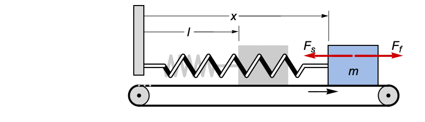
beltv[t_] = vb;
spring[x_] = k(l - x);
friction[v_] := -a(v - beltv[t]);sys := {m x''[t] == spring[x[t]] + friction[x'[t]], x[0] == l, x'[0] == 0};sol = DSolve[sys, x, t];{pos[m_, k_, a_, vb_, t_], vel[m_, k_, a_, vb_, t_]} = {x[t], x'[t]} /. sol[[1]]//FullSimplifyl = 1;
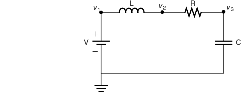
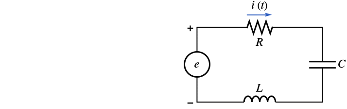
Manipulate[{Plot[{pos[m, k, a, vb, t]}, {t, 0, 2}, PlotRange -> All, PlotLabel -> "Position"], Plot[{vel[m, k, a, vb, t], vb}, {t, 0, 2}, PlotRange -> All, PlotLabel -> "Velocity"]}, {{m, 1, "mass of the block"}, 1, 10, 1}, {{k, 100, "spring constant"}, 100, 1000, 100}, {{vb, 1, "belt velocity"}, 1, 10, 1}, {{a, 5, "friction coefficient"}, 5, 45, 10}, SaveDefinitions -> True]接続に関するキルヒッホフ(Kirchhoff)の法則に加えて構成成分の諸法則を使って,時間

で適用される電圧
のステップインパルスに対するRLC回路の応答のシミュレーションを行う:
ClearAll[r, l, c];
vR[t_] := r iL[t];
vL[t_] := v1[t] - vR[t] - vC[t];
sys = {l iL'[t] == vL[t], c vC'[t] == iL[t]};v1[t_] := UnitStep[t - .01];
ic = {iL[0] == 0, vC[0] == 0};sol = DSolve[Flatten[{sys, ic}], {iL, vC}, t];{iL1[r_, c_, l_, t_], vC1[r_, c_, l_, t_]} = {iL[t], vC[t]} /. sol[[1]];Manipulate[{Plot[Evaluate[{v1[t], Re[vC1[r, c, l, t]]}], {t, 0, .03}, Filling -> {1 -> 0}, Ticks -> {Range[0.01, 0.03, 0.01], Automatic}, PlotRange -> All, PlotLabel -> "SubscriptBox[V, C][t]"], Plot[Evaluate[Re[iL1[r, c, l, t]]], {t, 0, .03}, Ticks -> {Range[0.01, 0.03, 0.01], Automatic}, PlotRange -> All, PlotLabel -> "SubscriptBox[I, L][t]"]}, {{r, 1, "R"}, 1, 10, 1}, {{l, 10^-2, "L"}, 10^-2, 5 10^-2, 10^-2}, {{c, 10^-4, "C"}, 10^-4, 5 10^-4, 10^-4}, SaveDefinitions -> True]水がパイプを通って1つのタンクから別のタンクに流れるときの,2つの円筒形タンクの水位の変化をモデル化する:
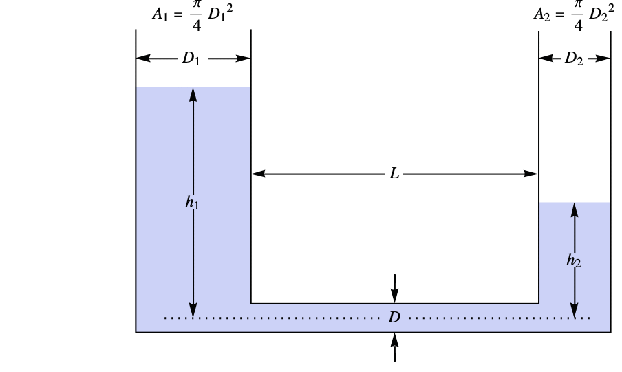
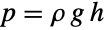
p1[t_] := ρ g h1[t];
p2[t_] := ρ g h2[t];Hagen–Poiseuille関係を使ってパイプの中のフローをモデル化する:

flowRate = (p1[t] - p2[t])(π pipeDia ^ 4) / (128 μ pipeLen);
massConservation = {a1 h1'[t] == -flowRate, a2 h2'[t] == flowRate};
ic = {h1[0] == 1, h2[0] == 0};sol = DSolve[Flatten[{massConservation, ic}], {h1, h2}, t]{h1[t_], h2[t_]} = {h1[t], h2[t]} /. sol[[1]];params = {pipeLen -> 0.1, pipeDia -> 0.2, a1 -> 1, a2 -> 1, ρ -> 0.2, μ -> 2 10 ^ -3, g -> 9.81};Plot[Evaluate[{h1[t], h2[t]} /. params], {t, 0, 15}, PlotRange -> All, PlotLegends -> {"SubscriptBox[h, 1][t]", "SubscriptBox[h, 2][t]"}]DSolve[{CaputoD[x[t], {t, 1.9}] + x[t] == 0, x[0] == 1, x'[0] == 0}, x[t], t]fracsol = Plot[x[t] /. %, {t, 0, 20}]dampedOsc = DSolve[{x''[t] + a x'[t] + x[t] == 0, x[0] == 1, x'[0] == 0}, x[t], t]//FullSimplify調和振動子についてのデータを減衰振動子の解にフィットして減衰係数
の対応する値を判定する:
data = Cases[InputForm[fracsol], Line[m_] :> m, -1][[1]];
fit = FindFit[data, x[t] /. dampedOsc, a, t]dampedsol = Plot[x[t] /. dampedOsc /. fit, {t, 0, 20}];
Show[fracsol, dampedsol]LCeqn[α_, l_, c_] = {CaputoD[i[t], {t, α}] + (1/l c)i[t] == 0, i[0] == 0.1, i'[0] == 0};LCsol[α_, l_, c_] := DSolve[LCeqn[α, l, c], i, t];LCsol[2, l, c]LCsol[1.9, l, c]Plot[Evaluate[i[t] /. {LCsol[2, 1, 1], LCsol[1.9, 1, 1], LCsol[1.8, 1, 1]}], {t, 0, 10}, PlotLegends -> {"α=2", "α=1.9", "α=1.8"}]RCeqn[α_, r_, c_] = {CaputoD[v[t], {t, α}] + (1/r c)v[t] == 0, v[0] == 20};RCsol[α_, r_, c_] := DSolve[RCeqn[α, r, c], v, t]RCsol[1, r, c]RCsol[0.9, r, c]Plot[Evaluate[v[t] /. {RCsol[1, 10, 1], RCsol[0.9, 10, 1], RCsol[0.8, 10, 1]}], {t, 0, 100}, PlotLegends -> {"α=1", "α=0.9", "α=0.8"}]ハイブリッド微分方程式 (8)
system = {x''[t] + .1x'[t] + x[t] == 0, x[0] == 1, x'[0] == 0};
control = WhenEvent[Mod[t, 1] == 0, x'[t] -> x'[t] + 1];sol = DSolve[{system, control}, x, {t, 0, 50}];Plot[Evaluate[{x[t], x'[t]} /. sol], {t, 0, 50}]sol = DSolve[{x''[t] + x[t] == 0, x[0] == 0, x'[0] == 1, WhenEvent[x[t] == 0, x'[t] -> -x'[t]]}, x, {t, 0, 4π}]Plot[{Sin[t], (x[t] /. sol)}, {t, 0, 4π}]c = .75;
sol = DSolve[{y''[t] == -9.8, y[0] == 13.5, y'[0] == 5, a[0] == 13, WhenEvent[y[t] - a[t] == 0, y'[t] -> -c y'[t]], WhenEvent[Mod[t, 1], a[t] -> a[t] - 1]}, {y, a}, {t, 0, 8}, DiscreteVariables -> {a}] ;Plot[Evaluate[{y[t], a[t]} /. sol], {t, 0, 8}, Filling -> {2 -> 0}, Exclusions -> None]正方形の箱の中で,側壁にあたるたびに方向を変えるボールをモデル化する:
sol = DSolve[{x'[t] == a[t], y'[t] == b[t], x[0] == 0, y[0] == 0, a[0] == 1, b[0] == 17 / 12, WhenEvent[x[t] ^ 2 == 1, a[t] -> -a[t]], WhenEvent[y[t] ^ 2 == 1, b[t] -> -b[t]]}, {x, y}, {t, 0, 50}, DiscreteVariables -> {a, b}];ParametricPlot[{x[t], y[t]} /. sol, {t, 0, 50}, Frame -> True, FrameTicks -> None, PlotRange -> 1, Axes -> False]system = {y'[t] == y[t] + u[t], y[0] == 1, u[0] == 0};
control = WhenEvent[Mod[t, 1] == 0, u[t] -> -2y[t]];DSolve[{system, control}, {y, u}, {t, 0, 20}, DiscreteVariables -> u];Plot[Evaluate[{u[t], y[t]} /. %], {t, 0, 10}, PlotRange -> {-6, 6}, Exclusions -> None]system = {x''[t] == u[t], x[0] == 1, x'[0] == 1, u[0] == -7};τ = 0.5;
control = WhenEvent[Mod[t, τ] == 0, u[t] -> -(1 / τ ^ 2)x[t] - (3 / (2τ))x'[t]];DSolve[{system, control}, {x, u}, {t, 0, 2}, DiscreteVariables -> u];Plot[Evaluate[{x[t], x'[t], u[t]} /. %], {t, 0, 2}, PlotRange -> All, Exclusions -> None]system = {x''[t] == u[t], x'[0] == x[0] == 0, u[0] == 1};kp = 1; td = 1;τ = 1; xref = 1;
control = WhenEvent[Mod[t, τ] == 0, u[t] -> kp(xref - x[t] - td x'[t])];DSolve[{system, control}, {x, u}, {t, 0, 12}, DiscreteVariables -> u];Plot[Evaluate[{xref, x[t], u[t]} /. %], {t, 0, 12}, Exclusions -> None]sol = DSolve[{a'[t] == -1 / 11u[t], a[0] == 1, u[0] == 1,
WhenEvent[a[t] < 0, u[t] -> 0]}, {a, u}, {t, 0, 15}, DiscreteVariables -> {u}]Plot[Evaluate[a[t] /. sol], {t, 0, 15}, PlotRange -> All]遅延微分方程式 (2)
遅延微分方程式によって支配されている動的な系における,カオスの発現を調べる:
sol = DSolve[{x'[t] == Sign[x[t - 2]] - x[t - 2], x[t /; t <= 0] == 0.1}, x,
{t, 0, 30}];ParametricPlot[Evaluate[{x[t - 2], x[t]} /. sol], {t, 2, 30}]f[λ_, μ_] := x[t] /. DSolve[{x'[t] == λ x[t] + μ x[t - 1], x[t /; t ≤ 0] == 1 - t}, x[t], {t, 0, 10}][[1]]Plot[Evaluate[{f[1 / 2, -1], f[-7 / 2, 4], f[-5, 4]}], {t, 0, 15}, Exclusions -> None]積分方程式 (4)
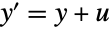
等時曲線問題では,ビーズ玉が,どこに置かれたものであれ,同じ時間で最下点まで落ちる下降曲線を求める必要がある.合計の下降時間を曲線の弧長と速度 v によって表すとアーベルの積分方程式
が与えられる.未知の関数
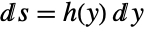
を関係
によって定義し,エネルギー方程式
の変換を使うと明示的な方程式が与えられる:
abeleqn = T == Subsuperscript[∫, 0, y](h[z]/Sqrt[2g]Sqrt[y - z])ⅆz;DSolveを使って積分方程式を解く:
DSolve[abeleqn, h[y], y]dxdy = Sqrt[h[y]^2 - 1] /. First[%]積分が実数値であるという仮定のもとに曲線を原点から始めて積分すると,
の関数としての
が与えられる:
x[y_] = Integrate[dxdy, {y, 0, y}, Assumptions -> (2 g T^2 /π^2y) > 1 && y > 0]
と
の値を代入し,ParametricPlotを使って最大等時曲線を表示する:
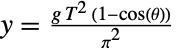
Show[ParametricPlot[{{x[y], y}, {-x[y], y}} /. {g -> 9.8, T -> 2}, {y, 0, (2(9.8)2^2/π^2)}], ImageSize -> Medium]変数
を変更すると,
の範囲での曲線の単純で特異ではないパラメータ化が与えられる:
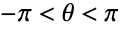
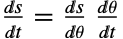
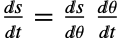
c[θ_] = (g T^2/π^2){Sin[θ] + θ, 1 - Cos[θ]} ;エネルギーの保存方程式とチェーン規則
を組み合せると,
の関数としての
について次の微分方程式が得られる:
FullSimplify[ (Sqrt[2g (Last[c[θMax]] - Last[c[θ]])] /Sqrt[c'[θ].c'[θ]]) , g > 0 && T > 0]teqn = θ'[t] == (% /. {θ -> θ[t], T -> 2});Θ[t_] = Table[NDSolveValue[{teqn, θ[0] == θMax}, θ[t], {t, 0, 4}], {θMax, {-2 Pi / 3, -Pi / 2, -Pi / 4, -Pi / 12}}];解をプロットするとすべてが2秒で最下点
に達することが分かる:
Plot[Evaluate[Θ[t]], {t, 0, 4}, PlotTheme -> "Scientific"]{cShape[t_], cBeads[t_]} = {c[t], c /@ Θ[t]} /. {T -> 2, g -> 9.8};
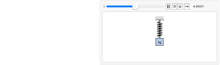
Animate@@{ParametricPlot[cShape[s] , {s, -Pi, Pi}, ImageSize -> Medium, Epilog -> {AbsolutePointSize[8], Point[cBeads[t]]}], {t, 0, 4, Appearance -> "Labeled"}, SaveDefinitions -> True, AnimationDirection -> ForwardBackward}3gの質量が付けられたバネ質量系は3dynes/cmのバネ定数と2g/sの減衰係数を持つ.
で質量が下方に押され,速度28cm/sで下向きに放たれる.
で
の力が質量に対して下向きにかかる.系の速度を時間の関数として求める.速度についての積分方程式は以下で与えられる:
ieqn = 3Derivative[1][v][t] + 2 v[t] + 40 Subsuperscript[∫, 0, t]v[m]ⅆm == 50 Cos[2 t];ic = v[0] == 28;DSolveを使って積分微分方程式を解く:
sol = DSolve[{ieqn, ic}, v[t], t]Plot[v[t] /. sol[[1]], {t, 0, 8}, PlotRange -> All, Filling -> Axis]
あるLRC回路の電源が
で与えられる.回路の抵抗は0.2
,インダクタンスは
ieqn = 5 Derivative[1][i][t] + 0.2 i[t] + (1/0.7)Subsuperscript[∫, 0, t]i[m]ⅆm == 2 Cos[t];ic = i[0] == 1;DSolveを使って積分微分方程式を解く:
sol = DSolve[{ieqn, ic}, i[t], t]//FullSimplify//ChopPlot[i[t] /. sol[[1]], {t, 0, 80}, PlotRange -> All, Filling -> Axis]線形ヴォルテラ積分方程式は線形微分方程式の初期値問題に等しい.この関係を次のヴォルテラ方程式について確かめる:
eqn = y[x] == x^3 + λSubsuperscript[∫, 0, x](t - x)y[t]ⅆt;DSolveを使って積分方程式を解く:
sol = DSolve[eqn, y[x], x]deqn = D[eqn, {x, 2}]init = {(eqn /. {x -> 0}), (D[eqn, x] /. {x -> 0})}DSolve[{deqn, init}, y[x], x]//SimplifyPlot[Table[y[x] /. %[[1]], {λ, 1, 3, 0.5}]//Evaluate, {x, 0, 20}, Filling -> Axis]従来の偏微分方程式 (5)
波動方程式を使って,固定長(例えば π)の紐の振動をモデル化する:
eqn = D[u[x, t], {t, 2}] == D[u[x, t], {x, 2}];bc = {u[0, t] == 0, u[π, t] == 0};ic = {u[x, 0] == Sin[m x], Derivative[0, 1][u][x, 0] == 0};dsol = DSolve[{eqn, bc, ic}, u, {x, t}, Assumptions -> Element[m, Integers]]sol1[x_, t_] = u[x, t] /. dsol[[1]]Table[Show[Plot[Table[sol1[x, t], {t, 0, 4}]//Evaluate, {x, 0, Pi}, Ticks -> False]], {m, 4}]ic = {u[x, 0] == x(π - x) ^ 2, Derivative[0, 1][u][x, 0] == 0};dsol = DSolve[{eqn, bc, ic}, u, {x, t}] /. {K[1] -> m}Inactive和から4項を抽出する:
sol[x_, t_] = TruncateSum[u[x, t] /. dsol[[1]], 4]Animate[Plot[sol[x, t], {x, 0, π}, PerformanceGoal -> "Quality", PlotRange -> {-5, 5}, ImageSize -> Medium], {t, 0, 12}, SaveDefinitions -> True]2Dで波動方程式を使って半径1の円形皮膜の振動をモデル化する:
eqn = r D[u[r, t], {t, 2}] == D[r D[u[r, t], r], r];bc = u[1, t] == 0;ic = {u[r, 0] == 0, Derivative[0, 1][u][r, 0] == 1};(dsol = DSolve[{eqn, bc, ic}, u[r, t], {r, t}])//TraditionalFormInactive和から項を抽出する:
h[r_, t_] = TruncateSum[u[r, t] /. dsol[[1]], 3]//N;Animate[Plot3D[h[r, t] /. {r -> Sqrt[x ^ 2 + y ^ 2]}, {x, y}∈Disk[], PlotRange -> {-1, 1}, Ticks -> None, Mesh -> True, MeshStyle -> {Red, Blue}, PlotStyle -> Yellow], {t, 0, 4}, SaveDefinitions -> True]熱伝導方程式を使って,長さ1の棒の中の熱の流れをモデル化する:
heqn = D[u[x, t], t] == D[u[x, t], {x, 2}];bc = {u[0, t] == 20, u[1, t] == 50};ic = u[x, 0] == 0;sol = DSolve[{heqn, bc, ic}, u[x, t], {x, t}]Inactive和から数項を抽出する:
approxsol = TruncateSum[u[x, t] /. sol[[1]], 3]//ExpandPlot[Table[approxsol, {t, 0.02, 0.5, 0.07}]//Evaluate, {x, 0, 1}, AxesOrigin -> {0, 0}]ssol = DSolve[{v''[x] == 0, v[0] == 20, v[1] == 50}, v[x], x]//ExpandPlot[v[x] /. ssol[[1]], {x, 0, 1}]heqn = D[u[x, t], t] == D[u[x, t], {x, 2}];bc = {Derivative[1, 0][u][0, t] == 0, Derivative[1, 0][u][1, t] == 0};ic = u[x, 0] == 20 + 80x;sol = DSolve[{heqn, bc, ic}, u[x, t], {x, t}]Inactive和から数項を抽出する:
approxsol = TruncateSum[u[x, t] /. sol[[1]], 4]//ExpandPlot[Table[approxsol, {t, 0.02, 0.9, 0.07}]//Evaluate, {x, 0, 1}, AxesOrigin -> {0, 0}, PlotRange -> All]
軸上の実部と虚部の値から始めて複素解析関数を構築する.実部と虚部(u と v)はコーシー・リーマン(Cauchy–Riemann)方程式を満足する:
creqns = {D[u[x, y], x] == D[v[x, y], y], D[v[x, y], x] == -D[u[x, y], y]};xvals = {u[x, 0] == x ^ 3, v[x, 0] == 0};sol = DSolve[{creqns, xvals}, {u, v}, {x, y}]Laplacian[{u[x, y], v[x, y]} /. sol[[1]], {x, y}]ContourPlot[{u[x, y], v[x, y]} /. sol[[1]], {x, -5, 5}, {y, -5, 5}, ContourStyle -> {Red, Blue}, PlotTheme -> "Marketing"]f[x_, y_] = u[x, y] + I v[x, y] /. sol[[1]](f[x, y]//Factor) /. {x + I y -> z}一般的な偏微分方程式 (5)
粘度パラメータが無限に小さくなる場合の,極限におけるバーガース方程式の平滑化解の衝撃波への進化を見る:
eqns = { D[u[x, t], t] + u[x, t]D[u[x, t], x] == ϵ D[u[x, t], {x, 2}] , u[x, 0] == Piecewise[{{1, x < 0}}]};dsol = DSolve[eqns, u, {x, t}]Plot3D[u[x, t] /. dsol[[1]] /. {ϵ -> 1 / 10}, {x, -2, 2}, {t, 0.001, 5}]Table[Plot3D[u[x, t] /. dsol[[1]] /. {ϵ -> 1 / 1000}, {x, -2, 2}, {t, 0.001, 5}, Exclusions -> All, Ticks -> None], {ϵ, {1 / 10, 1 / 100, 1 / 1000}}]//Quiet長さ d の一次元の箱の中で動くように条件付けられた電子は,端点にディリクレ条件がある自由シュレディンガー方程式に支配されている:
eqn = I ℏ D[ψ[x, t], t] == (-ℏ^2/2m) D[ψ[x, t], {x, 2}];
bcs = {ψ[0, t] == 0, ψ[d, t] == 0};DSolve[Join[{eqn}, bcs], ψ[x, t], {x, t}]和の中の各項は,正弦を初期状態として使うと確率密度定
が時間依存になるので,常状態と呼ばれる.例えば,以下のようになる:
sol1 = DSolve[Join[{eqn, ψ[x, 0] == Sqrt[(2/d)]Sin[Pi(x/d)]}, bcs], ψ[x, t], {x, t}]ρ1[x_, t_] = Simplify[ComplexExpand[Conjugate[ψ[x, t]]ψ[x, t] /. First[sol1]], d > 0]初期データの正規化は,密度の積分(どこかに粒子を発見する全確率)が1になるように選択される:
Integrate[ρ1[x, t], {x, 0, d}]上記以外の初期条件を使うと,たとえ2つの定常状態の和のように単純なものでも,結果として複雑な時間依存密度になる:
sol2 = DSolve[Join[{eqn, ψ[x, 0] == (1/Sqrt[d])Sin[Pi(x/d)] + (1/Sqrt[d])Sin[2Pi(x/d)]}, bcs], ψ[x, t], {x, t}]ρ2[x_, t_] = Simplify[ComplexExpand[Conjugate[ψ[x, t]]ψ[x, t] /. First[sol2]], d > 0]Integrate[ρ2[x, t], {x, 0, d}]電子質量と
の値をSI単位で入れ,d をよく使われる原子間距離の1nmに設定すると,次の密度関数になる:
ρe[x_, t_] = ρ2[x, t] /. {ℏ -> 1.055*^-34, m -> 9.109 * 10 ^ -31, d -> 10 ^ -9}Plot3D[ρe[x 10^-9, t 10^-15]10^-9, {x, 0, 1}, {t, 0, 3.66}, PlotTheme -> {"Grid", "LargeLabels"}, AxesLabel -> {"x (nm)", "t (fs)", "ρe (SuperscriptBox[nm, -1])"}, ImageSize -> Medium]グラフを確率密度の動画として見ると,電子の「中心」が箱の片側からもう片側に動くのが分かる:
Animate[Plot[ρe[x, t], {x, 0, 10 ^ -9}, PerformanceGoal -> -"Quality", PlotRange -> {0, 4*^9}, ImageSize -> Medium, AxesLabel -> {"x (m)", "ρe (SuperscriptBox[m, -1])"}], {t, 0, 3.66*^-15}, SaveDefinitions -> True]ブラック・ショールズモデルを使って,もとになっている資産価格と行使価格の両方が100ドル,安全金利5%,もとになっている資産価格のボラティリティが20%,満期1年の場合の,ヨーロッパバニラオプションの値を求める:
BlackScholesModel = {D[c[t, s], t] + 1 / 2σ ^ 2 s ^ 2 D[c[t, s], {s, 2}] + r s D[c[t, s], s] - r c[t, s] == 0, c[T, s] == Max[s - k, 0]};dsol = c[t, s] /. DSolve[BlackScholesModel, c[t, s], {t, s}][[1]]dsol /. {t -> 0, s -> 100, k -> 100, σ -> 0.2, T -> 1, r -> 0.05}FinancialDerivativeで与えられた値と比較する:
FinancialDerivative[{"European", "Call"}, {"StrikePrice" -> 100.00, "Expiration" -> 1}, {"InterestRate" -> 0.05, "Volatility" -> 0.2, "CurrentPrice" -> 100}]sol = DSolve[{D[f[x, y], x] == x y Cos[x y] + Sin[x y],
D[f[x, y], y] == -E^-y + x^2 Cos[x y]}, f, {x, y}]Plot3D[Table[f[x, y, z] /. sol[[1]] /. {C[1] -> k}, {k, 1, 22, 5}]//Evaluate, {x, 0, 10}, {y, 0, 2}, PlotRange -> All]コーシー問題を解き,スターリング数(Stirling)を生成する:
sol = u[x, y] /. DSolve[{(1 - x)D[u[x, y], x] == y u[x, y], u[0, y] == 1}, u, {x, y}][[1]]Table[(-1) ^ i SeriesCoefficient[ Series[sol, {x, 0, 10}, {y, 0, 4}], {10, i}]10!, {i, 4}]StirlingS1[10, Range[4]]特性と関係 (10)
DSolve[{y''[x] - y[x] == 0, y[0] == 1, y'[0] == 4}, y, x]Simplify[{y''[x] - y[x] == 0, y[0] == 1, y'[0] == 4} /. %]Integrateに相当する微分方程式:
DSolve[y'[x] == Exp[x ^ 2], y, x]Integrate[Exp[x ^ 2], x]NDSolveを使って数値解を求める:
exactsol = DSolve[{y''[x] + y[x] == 0, y[0] == 1, y'[0] == 0}, y, x]Table[y[x] /. exactsol[[1]], {x, -2., 2}]numsol = NDSolve[{y''[x] + y[x] == 0, y[0] == 1, y'[0] == 0}, y, {x, -2, 2}]Table[y[x] /. numsol[[1]], {x, -2., 2}]DEigensystemを使って固有値と固有関数を求める:
{ℒ, ℬ} = {-Laplacian[u[x], {x}], DirichletCondition[u[x] == 0, True]};DSolve[{u''[x] + λ u[x] == 0, u[0] == 0, u[π] == 0}, u[x], x]DEigensystem[{ℒ, ℬ}, u[x], {x, 0, Pi}, 3]DSolveを使ってインパルス応答を計算する:
DSolve[y'''[x] - 5y''[x] + 9y'[x] - 5y[x] == DiracDelta''[x] + 2DiracDelta'[x] + DiracDelta[x] && y[-1] == 0 && y'[-1] == 0 && y''[-1] == 0, y[x], x]//FullSimplifyInverseLaplaceTransformを使って同じ計算をする:
InverseLaplaceTransform[(s ^ 2 + 2s + 1/s ^ 3 - 5s ^ 2 + 9s - 5), s, x]//FullSimplifyDSolveは,解の規則を返す:
DSolve[{y'[x] == y[x], y[0] == 1}, y[x], x]DSolveValueは,解の式を返す:
DSolveValue[{y'[x] == y[x], y[0] == 1}, y[x], x]記号界が得られない場合は,N[DSolve[...]]を適用してNDSolveを呼び出す:
DSolve[{y''[x] + x ^ 2 y'[x] + Tan[y[x]] == 1, y[0] == 1, y'[0] == 1}, y, {x, 0, 1}]N[%]Table[y[x] /. %[[1]], {x, 0, 1, 0.2}]peqn = Laplacian[u[x, y], {x, y}] == 0;bc = {u[x, 0] == 0, u[x, 1] == 0, u[0, y] == y ^ 2 - y, u[1, y] == 0};u[x, y] /. DSolve[{peqn, bc}, u[x, y], {x, y}][[1]]Ω = Rectangle[{0, 0}, {1, 1}];rbc = DirichletCondition[u[x, y] == Piecewise[{{y ^ 2 - y, x == 0}}], True];u[x, y] /. DSolve[{peqn, rbc}, u, {x, y}∈Ω][[1]]DFixedPointsを使って2つの常微分方程式の系の固定点を求める:
DFixedPoints[{x'[t] == -x[t] - y[t] - 1, y'[t] == 2x[t] - y[t] + 5}, {x, y}, t]DStabilityConditionsを使って固定点の安定性を解析する:
DStabilityConditions[{x'[t] == -x[t] - y[t] - 1, y'[t] == 2x[t] - y[t] + 5}, {x, y}, t]sol = DSolve[{x'[t] == -x[t] - y[t] - 1, y'[t] == 2x[t] - y[t] + 5, x[0] == -2, y[0] == 1}, {x[t], y[t]}, t]//Simplifysol = DSolve[{x'[t] == -x[t] - y[t] - 1, y'[t] == 2x[t] - y[t] + 5, x[0] == 3, y[0] == -2}, {x[t], y[t]}, t]//SimplifyPlot[Evaluate[{x[t], y[t]} /. sol], {t, 0, 20}]sim = SystemModelSimulate[[image]]SystemModelPlot[sim]考えられる問題 (9)
sol = DSolve[y'[x] == f[x], y[x], x]sol /. f -> Function[x, 0]Activateを使って積分を評価する:
Activate[%]DSolve[x'[K] == K ^ K, x[K], K]DSolve[x'[C] == C ^ C, x[C], C]DSolve[x'[k] == k ^ k, x[k], k]DSolve[x'[c] == c ^ c, x[c], c]DSolve[{y'[x] ^ 2 == (1 - y[x] ^ 2)(1 - (1 / 2)y[x] ^ 2), y[0] == 0}, y, x]y[x_] := Cos[x]DSolve[{y'[x] == 0, y[0] == 1}, y, x]未知の関数についての定義をクリアすると,この問題は解決する:
Clear[y]DSolve[{y'[x] == 0, y[0] == 1}, y, x]ここでは,
が第2引数に含まれていないので,DSolveがエラーメッセージを出す:
DSolve[{y'[x] == 3y[x], z'[x] == 2 z[x], z[0] == 1, y[0] == 1}, y[x], x]DSolve[{y'[x] == 3y[x], z'[x] == 2 z[x], z[0] == 1, y[0] == 1}, {y[x], z[x]}, x]あるいは,DSolveValueを使って
についての解のみを得ることもできる:
DSolveValue[{y'[x] == 3y[x], z'[x] == 2 z[x], z[0] == 1, y[0] == 1}, y[x], x]DSolveは問題がベクトル方程式であると解釈できないので,この例は未評価で返される:
A = {{2, 0}, {-2, 0}};B = {3t, 4};eqn = x'[t] == A.x[t] + BDSolve[eqn, x∈Vectors[2], t]eqn1 = x'[t] + A.x[t] == BDSolve[eqn1, x∈Vectors[2], t]eqn1 /. %[[1]]//SimplifyCompleteIntegralは非線形偏微分方程式の完全積分を求める:
deqn = D[u[x, y], x] + D[u[x, y], y] ^ 2 == 3;CompleteIntegral[deqn, u[x, y], {x, y}]DSolveは同じ解を警告メッセージとともに返す:
DSolve[deqn, u[x, y], {x, y}]CompleteIntegralを使って線形偏微分方程式の完全積分を求める:
deqn = D[u[x, y], x] + 2D[u[x, y], y] == 1;CompleteIntegral[deqn, u[x, y], {x, y}]DSolveはこの偏微分方程式の一般解を返す:
DSolve[deqn, u[x, y], {x, y}]eqn = y''[x] + (k + g1 / (a + x)) y'[x] + (m + g2 / (a + x)) y[x] == 0;sol = DSolve[eqn, y[x], x]得られた解は.特定のパラメータ値
についての常微分方程式の一般解ではない:
y[x] /. sol[[1]] /. {g1 -> 0, g2 -> 0}//Simplifyこの場合の一般解は,まず方程式のパラメータ値に代入することで求められる:
DSolve[eqn /. {g1 -> 0, g2 -> 0}, y[x], x]おもしろい例題 (2)
DSolve[{x'[s] == Cos[t[s]], y'[s] == Sin[t[s]], t'[s] == s, x[0] == 0, y[0] == 0, t[0] == 0}, {x, y, t}, s]ParametricPlot[Evaluate[{x[s], y[s]} /. %], {s, -10, 10}]sol = DSolve[(-((192n(1 + n)x ^ 5) / (1 - x ^ 2) ^ 6) + (2496n(1 + n)x ^ 3) / (1 - x ^ 2) ^ 5 - (8160n ^ 2(1 + n) ^ 2x ^ 3) / (1 - x ^ 2) ^ 5 - (1632n(1 + n)x) / (1 - x ^ 2) ^ 4 + (7824n ^ 2(1 + n) ^ 2x) / (1 - x ^ 2) ^ 4 - (6912n ^ 3(1 + n) ^ 3x) / (1 - x ^ 2) ^ 4)y[x] + ((64x ^ 6) / (1 - x ^ 2) ^ 6 - (1824x ^ 4) / (1 - x ^ 2) ^ 5 + (8256n(1 + n)x ^ 4) / (1 - x ^ 2) ^ 5 + (2880x ^ 2) / (1 - x ^ 2) ^ 4 - (19200n(1 + n)x ^ 2) / (1 - x ^ 2) ^ 4 + (22896n ^ 2(1 + n) ^ 2x ^ 2) / (1 - x ^ 2) ^ 4 - 272 / (1 - x ^ 2) ^ 3 + (2208n(1 + n)) / (1 - x ^ 2) ^ 3 - (4384n ^ 2(1 + n) ^ 2) / (1 - x ^ 2) ^ 3 + (2304n ^ 3(1 + n) ^ 3) / (1 - x ^ 2) ^ 3) y'[x] + (-((2016x ^ 5) / (1 - x ^ 2) ^ 5) + (9408x ^ 3) / (1 - x ^ 2) ^ 4 - (19488n(1 + n)x ^ 3) / (1 - x ^ 2) ^ 4 - (3696x) / (1 - x ^ 2) ^ 3 + (12768n(1 + n)x) / (1 - x ^ 2) ^ 3 - (9408n ^ 2(1 + n) ^ 2x) / (1 - x ^ 2) ^ 3)y''[x] + ((4816x ^ 4) / (1 - x ^ 2) ^ 4 - (7168x ^ 2) / (1 - x ^ 2) ^ 3 + (9632n(1 + n)x ^ 2) / (1 - x ^ 2) ^ 3 + 616 / (1 - x ^ 2) ^ 2 - (1456n(1 + n)) / (1 - x ^ 2) ^ 2 + (784n ^ 2(1 + n) ^ 2) / (1 - x ^ 2) ^ 2)y'''[x] + (-((2800x ^ 3) / (1 - x ^ 2) ^ 3) + (1400x) / (1 - x ^ 2) ^ 2 - (1400n(1 + n)x) / (1 - x ^ 2) ^ 2) y''''[x] + ((560x ^ 2) / (1 - x ^ 2) ^ 2 - 70 / (1 - x ^ 2) + (56n(1 + n)) / (1 - x ^ 2))y'''''[x] - (42x y''''''[x]) / (1 - x ^ 2) + y'''''''[x] == 0, y, x]テクニカルノート
履歴
1991 で導入 (2.0) | 1996 で更新 (3.0) ▪ 2003 (5.0) ▪ 2014 (10.0) ▪ 2015 (10.3) ▪ 2016 (11.0) ▪ 2019 (12.0) ▪ 2021 (13.0) ▪ 2022 (13.1) ▪ 2022 (13.2) ▪ 2024 (14.1) ▪ 2025 (14.2) ▪ 2026 (15.0)
テキスト
Wolfram Research (1991), DSolve, Wolfram言語関数, https://reference.wolfram.com/language/ref/DSolve.html (2026年に更新).
CMS
Wolfram Language. 1991. "DSolve." Wolfram Language & System Documentation Center. Wolfram Research. Last Modified 2026. https://reference.wolfram.com/language/ref/DSolve.html.
APA
Wolfram Language. (1991). DSolve. Wolfram Language & System Documentation Center. Retrieved from https://reference.wolfram.com/language/ref/DSolve.html
BibTeX
@misc{reference.wolfram_2026_dsolve, author="Wolfram Research", title="{DSolve}", year="2026", howpublished="\url{https://reference.wolfram.com/language/ref/DSolve.html}", note=[Accessed: 15-September-2026]}
BibLaTeX
@online{reference.wolfram_2026_dsolve, organization={Wolfram Research}, title={DSolve}, year={2026}, url={https://reference.wolfram.com/language/ref/DSolve.html}, note=[Accessed: 15-September-2026]}