



RadialAxisPlot
RadialAxisPlot[{y1,y2,…,yn}]
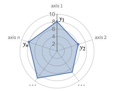
生成径向轴绘图,其中 yi 显示在径向轴上,在原点周围均匀排开.
RadialAxisPlot[{data1,data2,…}]
在轴上绘制多个数据组 datai.
更多信息和选项
- RadialAxisPlot 也称作雷达图、蜘蛛图或星图.
- RadialAxisPlot 通过将每个维度映射在一个轴上创建一个独特的图形,可用于可视化多维数据. 不同数据点的形状可相互进行对比.
- 数据值 yi 可以如下形式给出:
-
yi 实值数字 Quantity[yi,unit] 带有单位的量 - 与之前显示的形式不同的值 yi 会被看成缺失和不显示.
- datai 有如下形式和解释:
-
<"k1"y1,"k2"y2,…> 值 {y1,y2,…} {y1"lbl1",y2"lbl2",…}, {y1,y2,…}{"lbl1","lbl2",…} 带有标签 {lbl1,lbl2,…} 的值 {y1,y2,…} SparseArray 正常数组值 TimeSeries,EventSeries,… 时间序列数据中的值 QuantityArray 量值 WeightedData 无权重值 - RadialAxisPlot[Tabular[…]cspec] 使用列规范 cspec 从表格对象中提取并绘制数值.
- 下列形式的列规范 cspec 可用于绘制表格数据:
-
{coly1,…,colyn} 在每列的坐标轴上绘制 colyi - 以下装饰器 w 可用于 datai:
-
Annotation[datai,label] 为数据提供注解 Button[datai,action] 当点击数据时定义一个执行的动作 Callout[datai,label] 用标注函数为数据添加标签 Callout[datai,label,pos] 在相对位置 pos 处放置该标注函数 EventHandler[datai,events] 为数据定义一个通用数据处理器 Hyperlink[datai,uri] 将数据变为超链接 Labeled[datai,label] 为数据添加标签 Labeled[datai,label,pos] 将标签放于相对位置 pos Legended[datai,label] 在图例中识别数据 PopupWindow[datai,cont] 为数据附加一个弹出窗口 StatusArea[datai,label] 鼠标移动到数据上方时在状态区域显示 Style[datai,styles] 使用特定样式显示数据 Tooltip[datai,label] 为曲线附加一个提示工具 - 装饰器 w 可以用于不同层:
-
{…,w[yi],…} 在数据中封装值 yi {…,w[{xi,yi}],…} 封装点 {xi,yi} w[datai] 封装数据 w[{data1,…}] 封装数据组 datai w1[w2[…]] 使用嵌套装饰器 - Callout,Labeled 和 Placed 可使用下列位置 pos:
-
Automatic 自动放置的标签 Above, Below, Before, After 曲线周围的位置 {pos,epos} 位于曲线相对位置 pos 的标签中的 epos - RadialAxisPlot 和 Graphics 的选项相同,有下列添加和变化: [所有选项的列表]
-
Axes True 是否绘制轴 AxesOrigin Automatic 是否为轴定位 ColorFunction Automatic 如何决定线条的着色 ColorFunctionScaling True 是否将参数缩放至 ColorFunction Filling True 在每条线下填充 FillingStyle Automatic 填充使用的样式 GridLines Automatic 是否绘制网格线 GridLinesStyle Automatic 网格线使用的样式 Method Automatic 用何方法 PerformanceGoal $PerformanceGoal 尝试优化的性能方面 PlotLayout Automatic 如何定位数据 PlotLegends None 线条的图例 PlotMarkers Automatic 用来表示每个点的记号 PlotRange Automatic 想要包括的值的值域 PlotStyle Automatic 决定每条线样式的图形指令 PlotTheme $PlotTheme 绘图的整体主题 ScalingFunctions None 如何缩放单个坐标 - 从正 y 轴开始轴顺时针排列.
- 默认情况下,所有轴都有同样的绘图区域.
- 设置 AxesAutomatic,如果所有轴的缩放比例和绘图范围都一样,则只显示第一条轴. 如果有任何的不同,则会显示所有轴.
- 默认设置 PlotRangeAutomatic,所有轴都使用相同的绘图范围.
- PlotRangeAll 为每条轴都使用一个不同的绘图范围.
- 应用于每条轴的选项,如 Axes,Ticks 和 PlotRange,可有以下形式:
-
s 为所有轴使用设置 s {s1,…,sn} 使用每轴设置即第一条轴使用 s1,以此类推 {…,pats,…} 为位置匹配模式 pat 的轴使用设置 s - 设置 {…,pats,…},pat 可为任意模式. 第一个匹配到轴位置的模式会被使用. 如果没有任何模式匹配轴位置,则使用默认值.
- 供给 ColorFunction 的参数是 y1,y2,…,yn. 默认情况下,每条轴的颜色函数参数在 0 到 1 之间进行缩放.
- 在单个绘图面板中显示多个点的 PlotLayout 的可能设置包括:
-
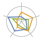
"Overlaid" 显示所有重叠的数据 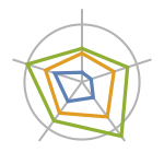
"Stacked" 堆叠数据 
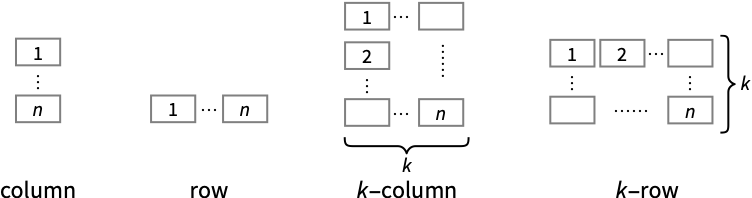
"Percentile" 堆叠并规范化数据 - 在多个绘图面板中显示单个点的 PlotLayout 的可能设置包括:
-
"Column" 在一列面板中使用单独的曲线 "Row" 在一行面板中使用单独的曲线 {"Column",k},{"Row",k} 使用 k 个列或行 {"Column",UpTo[k]},{"Row",UpTo[k]} 最多使用 k 列或行 - ColorData["DefaultPlotColors"] 给出 PlotStyle 使用的默认颜色序列.
所有选项的列表
范例
打开所有单元 关闭所有单元基本范例 (3)
RadialAxisPlot[{9, 7, 9, 5, 5, 7}]RadialAxisPlot[{{9, 7, 9, 5, 5, 7}, {6, 2, 3, 8, 8, 7}, {6, 8, 3, 4, 1, 9}}]使用 ColorFunction 可通过第一条轴上的值对线条添加样式:
RadialAxisPlot[RandomReal[{1, 10}, {5, 10}], ColorFunction -> (ColorData["Rainbow"][#]&), Filling -> False]范围 (23)
通用数据 (6)
通过将每个维度都放在同一个原点出发的轴上,RadialAxisPlot 可实现对多维度数据的可视化:
RadialAxisPlot[{9, 13, 5, 7, 3, 11}]自动 PlotRange 可在同一范围内显示每条轴:
RadialAxisPlot[{1, 5, 10, 15, 20, 25, 50, 100}]PlotRangeAll 将每条轴显示在自己的范围内:
RadialAxisPlot[{1, 5, 10, 15, 20, 25, 50, 100}, PlotRange -> All]RadialAxisPlot[{{9, 13, 5, 7, 3, 11}, {5, 9, 8, 13, 10, 9}, {6, 7, 4, 13, 3, 6}, {3, 13, 2, 12, 6, 11}}]RadialAxisPlot[{{6, 10, 5, 9, 7, 4}, {10, 5, 8, 6, 3}, {2, 5, 3}}]RadialAxisPlot[{{8, 3, 5, 6, Missing[], 9}, {2, 6, a, 9, 12, 5}, {6, I, 5, 9, 5, 7}}]表格数据 (1)
iris = ResourceData["Sample Tabular Data: Fisher Iris"]RadialAxisPlot[iris -> {"SepalLength", "SepalWidth", "PetalLength", "PetalWidth"}, AxesLabel -> {"SepalLength", "SepalWidth", "PetalLength", "PetalWidth"}]RadialAxisPlot[iris -> {"SepalLength", "SepalWidth", "PetalLength", "PetalWidth"}, AxesLabel -> {"SepalLength", "SepalWidth", "PetalLength", "PetalWidth"}, PlotRange -> All]特殊数据 (2)
使用 Quantity 可为数据添加单位:
RadialAxisPlot[{Quantity[Range[6], "Meters"], Quantity[Range[6], "Yards"], Quantity[Range[6], "Feet"]}, PlotRange -> Automatic]在 TimeSeries 中绘制值:
RadialAxisPlot[{TimeSeries[{19, 16, 9, 3, 7, 2, 17}, {"May 24, 1982"}],
	TimeSeries[{10, 19, 15, 3, 18, 17, 19}, {"May 24, 1982"}],
	TimeSeries[{10, 11, 17, 18, 8, 7, 19}, {"May 24, 1982"}]}]
Association 中的键自动用作轴标签:
RadialAxisPlot[{<|"a" -> 1, "b" -> 2, "c" -> 3|>, <|"a" -> 3, "b" -> 1, "c" -> 2|>, <|"a" -> 5, "b" -> 1, "c" -> 4|>}]数据装饰器 (4)
{RadialAxisPlot[{Style[{1, 3, 2, 4, 5}, Directive[Thick, Red]], {2, 4, 6, 2, 3}, {3, 1, 2, 1, 4}}],
RadialAxisPlot[Style[{{1, 3, 2, 4, 5}, {2, 4, 6, 2, 3}, {3, 1, 2, 1, 4}}, Directive[Thick, Red]]]}RadialAxisPlot[Style[{Style[{1, 3, 2, 4, 5}, Directive[Thick, Red]], {2, 4, 6, 2, 3}, {3, 1, 2, 1, 4}}, Directive[Dashed, Purple]]]使用 PopupWindow 可提供额外的向下钻取信息:
RadialAxisPlot[{Style[PopupWindow[{1, 3, 2, 4, 5}, RadialAxisPlot[{1, 3, 2, 4, 5}]], Red], {2, 4, 6, 2, 3}, {3, 1, 2, 1, 4}}]Button 可用于出发任何动作:
RadialAxisPlot[{Button[Style[{1, 3, 2, 4, 5}, Red], Print[RadialAxisPlot[{1, 3, 2, 4, 5}]]], {2, 4, 6, 2, 3}, {3, 1, 2, 1, 4}}]标签和图例 (6)
使用 LabelingFunction 为每个数据集添加单个标签:
RadialAxisPlot[RandomReal[1, {4, 5}], LabelingFunction -> (Callout[RandomWord[]]&)]使用提供给 LabelingFunction 的数据集指数构建标签:
labels = Table[RandomWord[], 4]RadialAxisPlot[RandomReal[1, {4, 5}], LabelingFunction -> (Callout[Part[labels, Last@#2]]&)]RadialAxisPlot[RandomReal[1, {4, 5}], LabelingFunction -> (Callout[Part[labels, Last@#2], Before]&)]使用 Callout 添加标签:
RadialAxisPlot[{Callout[{1, 3, 2, 4, 3}, "label"], {2, 4, 6, 2, 1}, {3, 1, 2, 1, 4}}]使用 PlotLegends 添加一个条形标签,代表 ColorFunction 中的颜色:
RadialAxisPlot[RandomReal[10, {5, 5}], ColorFunction -> "Rainbow", PlotLegends -> Automatic]RadialAxisPlot[RandomReal[10, {3, 5}], PlotLegends -> {"a", "b", "c"}]使用 Legended 添加图例:
RadialAxisPlot[{Legended[Style[{1, 3, 2, 4, 3}, Red], "label"], {2, 4, 6, 2, 1}, {3, 1, 2, 1, 4}}]演示 (4)
RadialAxisPlot[RandomReal[10, {3, 5}]]RadialAxisPlot[RandomReal[10, {3, 5}], PlotStyle -> {RGBColor[0.8, 0.1, 0.1], Darker@Green, Hue[0.7]}]RadialAxisPlot[RandomReal[10, {3, 5}], PlotTheme -> "Marketing"]RadialAxisPlot[RandomReal[10, {3, 5}], PlotLegends -> Automatic]选项 (53)
AspectRatio (3)
默认情况下,RadialAxisPlot 使用相同的宽度和高度:
RadialAxisPlot[{{9, 7, 9, 5, 5, 7}, {6, 2, 3, 8, 8, 7}, {6, 8, 3, 4, 1, 9}}]RadialAxisPlot[{{9, 7, 9, 5, 5, 7}, {6, 2, 3, 8, 8, 7}, {6, 8, 3, 4, 1, 9}}, AspectRatio -> (1/2)]AspectRatioFull 调整高度和宽度,以紧密适应其他结构:
plot = RadialAxisPlot[{{9, 7, 9, 5, 5, 7}, {6, 2, 3, 8, 8, 7}, {6, 8, 3, 4, 1, 9}}, AspectRatio -> Full];{Framed[Pane[plot, {50, 100}]], Framed[Pane[plot, {100, 100}]], Framed[Pane[plot, {100, 50}]]}Axes (4)
RadialAxisPlot[{8, 4, 7, 6, 9, 7, 5, 5, 1}]RadialAxisPlot[{8, 4, 7, 6, 9, 7, 5, 5, 1}, PlotRange -> All]RadialAxisPlot[{8, 4, 7, 6, 9, 7, 5, 5, 1}, PlotRange -> {3 -> {0, 15}}]RadialAxisPlot[{8, 4, 7, 6, 9, 7, 5, 5, 1}, Axes -> {True, False, True, Automatic}]RadialAxisPlot[{8, 4, 7, 6, 9, 7, 5, 5, 1}, Axes -> {1 -> True, _ -> False}]AxesLabel (2)
AxesOrigin (3)
RadialAxisPlot[{{3, 6, 6, 8, 2, 6}, {6, 3, 0, 1, 7, 5}}, AxesOrigin -> Pi / 3]RadialAxisPlot[{{3, 6, 6, 8, 2, 6}, {6, 3, 0, 1, 7, 5}}, AxesOrigin -> .5]Table[RadialAxisPlot[{{3, 6, 6, 8, 2, 6}, {6, 3, 0, 1, 7, 5}}, AxesOrigin -> {Pi / 3, o}], {o, {-1, 1}}]RadialAxisPlot[{{3, 6, 6, 8, 2, 6}, {6, 3, 0, 1, 7, 5}}, AxesOrigin -> {{Pi / 3, -1}, 0.2}]AxesStyle (3)
RadialAxisPlot[{3, 9, 9, 8, 4}, Axes -> True, AxesStyle -> Red]RadialAxisPlot[{3, 9, 9, 8, 4}, Axes -> True, AxesStyle -> {{Thick, Red}, {Thick, Green}, {Thick, Blue}, {Thick, Yellow}, {Thick, Purple}}]RadialAxisPlot[{3, 9, 9, 8, 4}, Axes -> True, AxesStyle -> Red, LabelStyle -> Green]ColorFunction (1)
ColorFunctionScaling (1)
Filling (6)
RadialAxisPlot[{{3, 9, 9, 7, 2}, {8, 10, 0, 6, 7}, {7, 10, 2, 4, 3}}]RadialAxisPlot[{{3, 9, 9, 7, 2}, {8, 10, 0, 6, 7}, {7, 10, 2, 4, 3}}, PlotLayout -> "Stacked"]RadialAxisPlot[{{3, 9, 9, 7, 2}, {8, 10, 0, 6, 7}, {7, 10, 2, 4, 3}}, Filling -> None]RadialAxisPlot[{{10, 14, 15, 11, 1, 12, 4, 13, 8, 7, 3, 5, 6, 2, 9}, {1, 2, 3, 11, 15, 7, 5, 14, 6, 12, 9, 10, 13, 8, 4}}, Filling -> {1 -> {2}}]RadialAxisPlot[{{10, 14, 15, 11, 1, 12, 4, 13, 8, 7, 3, 5, 6, 2, 9}, {1, 2, 3, 11, 15, 7, 5, 14, 6, 12, 9, 10, 13, 8, 4}}, Filling -> {2 -> {{1}, Red}}]RadialAxisPlot[RandomReal[{-5, 10}, {3, 10}], PlotLayout -> "Stacked"]FillingStyle (1)
Frame (2)
FrameStyle (2)
RadialAxisPlot[RandomInteger[10, {4, 5}], Frame -> True, FrameStyle -> Red]RadialAxisPlot[{{9, 7, 9, 5, 5, 7}, {6, 2, 3, 8, 8, 7}, {6, 8, 3, 4, 1, 9}}, AxesOrigin -> {{Automatic, Automatic}, 0.2}, Frame -> True, FrameStyle -> {Directive[Red, Thick], Blue}]GridLines (3)
RadialAxisPlot[RandomInteger[10, {4, 5}], GridLines -> Automatic]RadialAxisPlot[RandomInteger[10, {4, 5}], GridLines -> {2, 4, 10}]Table[RadialAxisPlot[RandomInteger[10, {4, 5}], GridLines -> shape, PlotLabel -> shape], {shape, {"Polygon", "Circle"}}]GridLinesStyle (1)
ImageSize (7)
使用命名尺寸,例如 Tiny、Small、Medium 和 Large:
{RadialAxisPlot[{{9, 7, 9, 5, 5, 7}, {6, 2, 3, 8, 8, 7}, {6, 8, 3, 4, 1, 9}}, ImageSize -> Tiny], RadialAxisPlot[{{9, 7, 9, 5, 5, 7}, {6, 2, 3, 8, 8, 7}, {6, 8, 3, 4, 1, 9}}, ImageSize -> Small]}{RadialAxisPlot[{{9, 7, 9, 5, 5, 7}, {6, 2, 3, 8, 8, 7}, {6, 8, 3, 4, 1, 9}}, ImageSize -> 150], RadialAxisPlot[{{9, 7, 9, 5, 5, 7}, {6, 2, 3, 8, 8, 7}, {6, 8, 3, 4, 1, 9}}, AspectRatio -> 1.5, ImageSize -> 150]}{RadialAxisPlot[{{9, 7, 9, 5, 5, 7}, {6, 2, 3, 8, 8, 7}, {6, 8, 3, 4, 1, 9}}, ImageSize -> {Automatic, 150}], RadialAxisPlot[{{9, 7, 9, 5, 5, 7}, {6, 2, 3, 8, 8, 7}, {6, 8, 3, 4, 1, 9}}, AspectRatio -> 2, ImageSize -> {Automatic, 150}]}{RadialAxisPlot[{{9, 7, 9, 5, 5, 7}, {6, 2, 3, 8, 8, 7}, {6, 8, 3, 4, 1, 9}}, ImageSize -> UpTo[200]], RadialAxisPlot[{{9, 7, 9, 5, 5, 7}, {6, 2, 3, 8, 8, 7}, {6, 8, 3, 4, 1, 9}}, AspectRatio -> 2, ImageSize -> UpTo[200]]}RadialAxisPlot[{{9, 7, 9, 5, 5, 7}, {6, 2, 3, 8, 8, 7}, {6, 8, 3, 4, 1, 9}}, ImageSize -> {200, 200}, Background -> StandardGray]设置 AspectRatioFull 将填充可用空间:
RadialAxisPlot[{{9, 7, 9, 5, 5, 7}, {6, 2, 3, 8, 8, 7}, {6, 8, 3, 4, 1, 9}}, AspectRatio -> Full, ImageSize -> {200, 200}, Background -> StandardGray]{RadialAxisPlot[{{9, 7, 9, 5, 5, 7}, {6, 2, 3, 8, 8, 7}, {6, 8, 3, 4, 1, 9}}, ImageSize -> {UpTo[150], UpTo[100]}], RadialAxisPlot[{{9, 7, 9, 5, 5, 7}, {6, 2, 3, 8, 8, 7}, {6, 8, 3, 4, 1, 9}}, AspectRatio -> 2, ImageSize -> {UpTo[150], UpTo[100]}]}Framed[Pane[RadialAxisPlot[{{9, 7, 9, 5, 5, 7}, {6, 2, 3, 8, 8, 7}, {6, 8, 3, 4, 1, 9}}, ImageSize -> Full, Background -> StandardGray], {200, 100}]]Framed[Pane[RadialAxisPlot[{{9, 7, 9, 5, 5, 7}, {6, 2, 3, 8, 8, 7}, {6, 8, 3, 4, 1, 9}}, AspectRatio -> Full, ImageSize -> {Scaled[0.5], Scaled[0.5]}, Background -> StandardGray], {200, 200}]]PlotLayout (4)
RadialAxisPlot[{{10, 7, 0, 2, 3, 10}, {3, 10, 4, 3, 10, 0}, {3, 0, 3, 4, 3, 3}, {0, 0, 0, 6, 8, 10}}]RadialAxisPlot[{{10, 7, 0, 2, 3, 10}, {3, 10, 4, 3, 10, 0}, {3, 0, 3, 4, 3, 3}, {0, 0, 0, 6, 8, 10}}, PlotLayout -> "Stacked"]RadialAxisPlot[RandomInteger[{-5, 10}, {4, 6}], PlotLayout -> "Stacked"]RadialAxisPlot[RandomInteger[{-5, 10}, {3, 6}], PlotLayout -> "Row"]RadialAxisPlot[RandomInteger[{-5, 10}, {3, 6}], PlotLayout -> "Column"]PlotMarkers (2)
PlotRange (3)
data = RandomInteger[10, {4, 5}];RadialAxisPlot[data]RadialAxisPlot[data, PlotRange -> All]RadialAxisPlot[RandomInteger[10, {4, 5}], PlotRange -> {0, 20}]RadialAxisPlot[RandomInteger[10, {4, 5}], PlotRange -> {1 -> {0, 15}, _ -> {0, 10}}]PlotRangePadding (4)
RadialAxisPlot[{{9, 8, 9, 7, 7}, {3, 0, 3, 10, 6}}]RadialAxisPlot[{{9, 8, 9, 7, 7}, {3, 0, 3, 10, 6}}, PlotRangePadding -> None]RadialAxisPlot[{{9, 8, 9, 7, 7}, {3, 0, 3, 10, 6}}, PlotRangePadding -> 4]RadialAxisPlot[{{9, 8, 9, 7, 7}, {3, 0, 3, 10, 6}}, PlotRangePadding -> Scaled[0.2]]应用 (1)
RadialAxisPlot 本质善于可视化体育数据. 比如,可视化 2018-2019 全赛季 NBA 球员的表现:
headers = {"Rk", "Player", "Pos", "Age", "Tm", "G", "GS", "MP", "FG", "FGA", "FG%", "3P", "3PA", "3P%", "2P", "2PA", "2P%", "FT", "FTA", "FT%", "ORB", "DRB", "TRB", "AST", "STL", "BLK", "TOV", "PF", "PTS"};
data = IconizedObject[«Player Data»];assocData = Dataset[AssociationThread[headers, #]& /@ data];
assocData = Select[assocData, And[#["MP"] / #["G"] > 24, #["G"] > 42]&];Length[assocData]Select[assocData, #Player == "Devin Booker"&]vals = {"2P", "3P", "PTS", "TRB", "AST"};
labels = {"2 Pointers Made", "3 Pointers Made", "Points", "Rebounds", "Assists"};avgs = Mean@assocData[[All, vals]];使用 Manipulate 创建一个可以在每个球员中切换的界面,并使用 RadialAxisPlot 可视化他们的表现和平均值的对比:
Manipulate[
	RadialAxisPlot[
	{
	IconizedObject[«avgs»],
	Normal[Select[IconizedObject[«assocData»], #Player == player&][[1]]][[IconizedObject[«vals»]]]
	},
	PlotRange -> {1 -> {0, 10}, 2 -> {0, 4}, 3 -> {0, 40}, 4 -> {0, 20}, 5 -> {0, 10}},
	PlotLegends -> {"League Average", player},
	AxesLabel -> IconizedObject[«labels»],
	ImageSize -> 400
],
	{{player, "Devin Booker"}, assocData[All, "Player"]//Normal}
	]
属性和关系 (4)
RadialAxisPlot 在多个径向轴上绘制多维度点:
RadialAxisPlot[{{1, 1, 1, 1, 1}, {1, 2, 3, 4, 5}, {5, 5, 5, 5, 5}}]ListPolarPlot 在极坐标上绘制多个点:
ListPolarPlot[{{1, 1, 1, 1, 1}, {1, 2, 3, 4, 5}, {5, 5, 5, 5, 5}}, Joined -> True]ParallelAxisPlot 在多个平行轴上绘制多维点:
{RadialAxisPlot[{{1, 1, 1, 1, 1}, {1, 2, 3, 4, 5}, {5, 5, 5, 5, 5}}], ParallelAxisPlot[{{1, 1, 1, 1, 1}, {1, 2, 3, 4, 5}, {5, 5, 5, 5, 5}}]}RadialAxisPlot 使用多个轴绘制单个点:
RadialAxisPlot[{1, 2, 3}]AngularGauge 在单个轴上绘制多个值:
AngularGauge[{1, 2, 3}, {0, 3}]PieChart 将值显示为整体的一部分:
{RadialAxisPlot[{1, 2, 3}], PieChart[{1, 2, 3}]}巧妙范例 (1)
使用 RadialGradientFilling 创建一个高度风格化的填充:
RadialAxisPlot[RandomReal[{0.5, 2}, 8], FillingStyle -> RadialGradientFilling[{ImageScaled[0], ImageScaled[0.5], ImageScaled[1]} -> {Red, Purple, Blue}], Method -> {"AxesInFront" -> True, "GridLinesInFront" -> True}]文本
Wolfram Research (2020),RadialAxisPlot,Wolfram 语言函数,https://reference.wolfram.com/language/ref/RadialAxisPlot.html (更新于 2025 年).
CMS
Wolfram 语言. 2020. "RadialAxisPlot." Wolfram 语言与系统参考资料中心. Wolfram Research. 最新版本 2025. https://reference.wolfram.com/language/ref/RadialAxisPlot.html.
APA
Wolfram 语言. (2020). RadialAxisPlot. Wolfram 语言与系统参考资料中心. 追溯自 https://reference.wolfram.com/language/ref/RadialAxisPlot.html 年