



RectangleChart
RectangleChart[{{x1,y1},{x2,y2},…}]
绘制一个矩形图表,其中竖条的宽度为 xi,高度为 yi.
RectangleChart[{…,wi[{xi,yi},…],…,wj[{xi,yj},…],…}]
绘制一个矩形图表,其中竖条的特性由符号封装 wk 定义.
RectangleChart[{data1,data2,…}]
根据多个数据集 datai 绘制矩形图表.
更多信息和选项
- 可用下列形式给出 RectangleChart 的数据元素:
-
{xi,yi} 竖条自身的宽度和高度 {Quantity[xi,ux],Quantity[yi,uy]} 带有单位的竖条的宽度和高度 wi[{xi,yi},…] 大小为 {xi,yi}、封装为 wi 的竖条 formi->mi 具有元数据 mi 的竖条形式 - 没有按这些形式给出的数据在矩形图表的形成过程中被忽略.
- 可用下列形式给出 RectangleChart 中的数据集:
-
{e1,e2,…} 有封装或无封装的元素列表 <k1{x1,y1},k2{x2,y2},…> 由键和值组成的关联 TimeSeries[…],EventSeries[…],TemporalData[…] 时间序列、事件序列和时间数据 WeightedData[…] 扩展数据集 w[{e1,e2,…},…] 应用到整个数据集的封装 w[{data1,data2,…},…] 应用到所有数据集中封装 - RectangleChart[objcspec] 用列指定 cspec 从 Tabular、TimeSeries 或 EventSeries 对象 obj 中提取值并绘制.
- 可使用以下形式的列指定 cspec 来绘制表格数据:
-
{colx,coly} 绘制列 y 与 x {{colx1,coly1},{colx2,coly2},…} 绘制列 y1 与 x1,y2 与 x2、… - 可对图表元素应用以下封装:
-
Annotation[e,label] 提供注解 Button[e,action] 定义元素被点击时要执行的操作 Callout[e,label] 显示元素及其标注 (callout) EventHandler[e,…] 定义元素的通用事件处理程序 Hyperlink[e,uri] 把元素变为超链接 Labeled[e,…] 显示元素及其标签 Legended[e,…] 在图例中显示元素的特点 Mouseover[e,over] 指定鼠标滑过元素时元素显示的形式 PopupWindow[e,cont] 为元素添加弹出窗口 StatusArea[e,label] 当鼠标悬停时在状态栏中显示 Style[e,opts] 用指定的样式显示元素 Tooltip[e,label] 为元素添加提示条 - 在 RectangleChart 中,Labeled ,Callout 和 Placed 可使用以下位置:
-
Top,Bottom,Left,Right,Center 竖条内的位置 Above,Below, Before, After 竖条外的位置 Axis 竖条起始的轴 {{bx,by},{lx,ly}} 竖条中的缩放位置 {bx,by} 处的标签中的缩放位置{lx,ly} - RectangleChart 有和 Graphics 相同的选项,并增加下列变化: [所有选项的列表]
-
AspectRatio 1/GoldenRatio 整体的高宽比 Axes True 是否绘制轴 BarOrigin Bottom 竖条的原点 BarSpacing Automatic 竖条间的间距 ChartElementFunction Automatic 如何产生竖条的原始图形 ChartElements Automatic 每个竖条使用的图形 ColorFunction Automatic 如何为竖条着色 ColorFunctionScaling True 是否归一化传递给 ColorFunction 的参数 LabelingFunction Automatic 如何标注竖条 LabelingSize Automatic 标注和标签的最大尺寸 LegendAppearance Automatic 图例的整体外观 PerformanceGoal $PerformanceGoal 优化的目标 PlotInteractivity $PlotInteractivity 是否允许出现互动元素 PlotLabels None 直条的类别标签 PlotLayout Automatic 使用的整体布局 PlotLegends None 数据元素和数据集的图例 PlotStyle Automatic 直条的样式 PlotTheme $PlotTheme 图表的整体主题 ScalingFunctions None 如何缩放单个坐标 TargetUnits Automatic 图表中显示的单位 - PlotLayout 的以下设置可用于显示多个数据集:
-
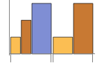
"Grouped" 分离每个数据集的数据 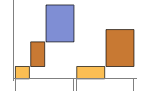
"Stepped" 累积和分离每个数据集的数据 - 在不同面板中显示单个数据集的 PlotLayout 的可能设置包括:
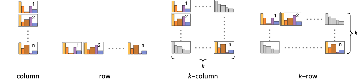
-
"Column" 在一列面板中用独立的图表显示 "Row" 在一行面板中用独立的图表显示 {"Column",k},{"Row",k} 使用 k 行或列 {"Column",UpTo[k]},{"Row",UpTo[k]} 最多使用 k 行或列 - PlotLegends 的典型设置包括:
-
None 无图例 Automatic 自动确定图例 {lbl1,lbl2,…} 用 lbl1、lbl2、… 作为图例的标签 Placed[lspec,…] 指定图例的放置 - PlotStylesty 指定每组数据使用的样式. 可能的设置包括:
-
{sty1,sty2,…} 针对各个数据集的一系列样式 <"key"val,…> 针对不同层级的数据的样式元素 - 接受的键有:
-
"Base" 所有直条的整体样式 "Elements" 针对每组数据中的元素 yi 的样式列表 "Groups" 针对每组数值 datai 的样式列表 - ColorData["DefaultChartColors"] 给出 PlotStyle 使用的默认颜色序列.
- ChartElementFunction 的参数是竖条区域{{xmin,xmax},{ymin,ymax}},数据值 {xi,yi} 和数据集的嵌套列表中每层的元数据 {m1,m2,…}.
- ChartElementFunction 的内置列表可以从 ChartElementData["RectangleChart"] 得到.
- ColorFunction 的参数是 xi 和 yi.
- RectangleChart 中选项和其它结构的样式或其它设置按照 PlotStyle、ColorFunction、Style、其它包装、ChartElements 和 ChartElementFunction 顺序作用,后面的设置会屏蔽之前的设置.
所有选项的列表
范例
打开所有单元 关闭所有单元基本范例 (4)
RectangleChart[{{1, 1}, {1, 2}, {2, 3}}]RectangleChart[{{{1, 1}, {1, 2}, {2, 3}}, {{3, 2}, {1, 3}, {2, 1}}}]RectangleChart[{{{1, 1}, {1, 2}, {2, 3}}, {{3, 2}, {1, 3}, {2, 1}}}, ChartLayout -> "Row"]data = {{{1, 1}, {1, 2}, {2, 3}}, {{1, 1}, {2, 1}}};RectangleChart[data, PlotLabels -> <|"Elements" -> {"a", "b", "c"}|>]RectangleChart[data, PlotLegends -> <|"Elements" -> {"a", "b", "c"}|>]RectangleChart[Tuples[{1, 2}, 2], PlotStyle -> {RGBColor[0.237736, 0.340215, 0.575113], RGBColor[0.33311066666666667, 0.5032283333333333, 0.26154733333333335], RGBColor[0.8562609999999999, 0.742794, 0.31908333333333333], RGBColor[0.72987, 0.239399, 0.230961]}]RectangleChart[Tuples[{1, 2}, 2], ChartElements -> {[image], {All, 1}}]RectangleChart[Tuples[{1, 2}, 2], ChartElementFunction -> "GlassRectangle", PlotStyle -> {RGBColor[0.761959, 0.470832, 0.940597], RGBColor[0.927848, 0.742785, 0.6151383333333333], RGBColor[0.929162, 0.95034, 0.6648153333333333], RGBColor[0.431296, 0.709773, 0.927077]}]范围 (41)
数据和布局 (13)
RectangleChart[{{{1, 1}, {1, 1}, {1, 1}}, {{2, 2}, {2, 2}, {2, 2}}}]RectangleChart[{{{1, 1}, {1, 2}, {2, 3}}, {{1, 1}, {2, 1}}}]RectangleChart[{{{1, 1}, Missing[], {1, 1}, {1, 1}}, {{2, 2}, 1 + I, {2, 2}}, {foo, {3, 3}}}]RectangleChart[{{Quantity[3, "Seconds"], Quantity[2, "Meters"]}, {Quantity[8, "Seconds"], Quantity[5, "Meters"]}, {Quantity[2, "Seconds"], Quantity[3, "Meters"]}, {Quantity[1, "Seconds"], Quantity[3, "Meters"]}, {Quantity[8, "Seconds"], Quantity[7, "Meters"]}, {Quantity[7, "Seconds"], Quantity[1, "Meters"]}}, AxesLabel -> Automatic, BarSpacing -> None, Ticks -> True]RectangleChart[{{Quantity[3, "Seconds"], Quantity[2, "Meters"]}, {Quantity[8, "Seconds"], Quantity[5, "Meters"]}, {Quantity[2, "Seconds"], Quantity[3, "Meters"]}, {Quantity[1, "Seconds"], Quantity[3, "Meters"]}, {Quantity[8, "Seconds"], Quantity[7, "Meters"]}, {Quantity[7, "Seconds"], Quantity[1, "Meters"]}}, AxesLabel -> Automatic, BarSpacing -> None, Ticks -> True, TargetUnits -> {"Minutes", "Feet"}]忽略 TimeSeries、EventSeries 和 TemporalData 中的时间戳:
RectangleChart[TimeSeries[{{19, 16}, {9, 3}, {7, 2}, {17, 5}}, {"May 24, 1982"}]]RectangleChart[<|"a" -> {1, 1}, "b" -> {1, 2}, "c" -> {2, 1}, "d" -> {2, 2}|>]RectangleChart[<|"a" -> {1, 1}, "b" -> {1, 2}, "c" -> {2, 1}, "d" -> {2, 2}|>, PlotLabels -> Automatic]RectangleChart[<|"a" -> {1, 1}, "b" -> {1, 2}, "c" -> {2, 1}, "d" -> {2, 2}|>, PlotLabels -> Callout[Automatic, Above]]RectangleChart[<|"a" -> {1, 1}, "b" -> {1, 2}, "c" -> {2, 1}, "d" -> {2, 2}|>, PlotLegends -> Automatic, PlotStyle -> {RGBColor[0.65, 0., 0.], RGBColor[0.0504678, 0.526626, 0.627561], RGBColor[0.752461, 0.362306, 0.125339], RGBColor[0.435888, 0.259065, 0.71028]}]RectangleChart[<|"group a" -> <|"a" -> {1, 2}, "b" -> {2, 1}|>, "group b" -> <|"a" -> {1, 1}, "b" -> {2, 2}|>|>, PlotLegends -> Automatic]忽略 WeightedData 中的权值;
RectangleChart[WeightedData[{{1, 1}, {2, 1}, {3, 2}, {4, 3}, {5, 5}}, {0.5, 0.2, 0.1, 0.2, 0.3}]]Table[RectangleChart[Tuples[{1, 2}, 2], ChartLayout -> l], {l, {"Grouped", "Stepped"}}]RectangleChart[{IconizedObject[«data #1»], IconizedObject[«data #2»], IconizedObject[«data #3»]}, ImageSize -> Medium, ChartLayout -> "Row"]RectangleChart[{IconizedObject[«data #1»], IconizedObject[«data #2»], IconizedObject[«data #3»]}, ImageSize -> Medium, ChartLayout -> "Column"]RectangleChart[{IconizedObject[«data #1»], IconizedObject[«data #2»], IconizedObject[«data #3»], IconizedObject[«data #4»]}, ImageSize -> Medium, ChartLayout -> {"Row", 2}]Table[RectangleChart[{{1, 1}, {1, 2}, {2, 3}}, BarOrigin -> o, PlotLabel -> o], {o, {Bottom, Left, Top, Right}}]Table[RectangleChart[Tuples[{1, 2}, 2], BarSpacing -> s, PlotLabel -> s, PlotStyle -> Opacity[0.8]], {s, {Automatic, {0, 1}, {-0.3, 1}}}]表格数据 (3)
tabdata = AggregateRows[Tabular[ResourceData["Sample Data: 1993 US Cars"]], {"AvgPrice" -> (Mean[#AvgPrice]&), "TotalCars" -> (Length[#AvgPrice]&), "AvgWeight" -> (Mean[#Weight]&), "AvgFuelTankCap" -> (Mean[#FuelTankCapacity]&)}, {"Type"}]RectangleChart[tabdata -> {"TotalCars", "AvgPrice"}, PlotLabels -> Normal[tabdata[All, "Type"]]]绘制 TimeSeries 或 EventSeries 中所有分量的值:
RectangleChart[TimeSeries[TimeEventSeries`TimestampData[Association["UniformlySpacedQ" -> True, "Count" -> 5,
   "Endpoints" -> TabularColumn[Association[
      "Data" -> {2, {{NumericArray[{20563, -2147483648}, "Integer32"], {},
          DataStructure["BitVec ...   {{TabularColumn[Association["Data" -> {{1, 1, 2, 5, 8}, {}, None},
           "ElementType" -> "Integer64"]], TabularColumn[Association[
           "Data" -> {{2, 2, 16, 17, 17}, {}, None}, "ElementType" -> "Integer64"]]}}]]]],
 Association[]]]
绘制 TimeSeries 或 EventSeries 中一组分量的值:
ts = TimeSeries[TimeEventSeries`TimestampData[Association["UniformlySpacedQ" -> True, "Count" -> 5,
   "Endpoints" -> TabularColumn[Association[
      "Data" -> {2, {{NumericArray[{20563, -2147483648}, "Integer32"], {},
          DataStructure["BitVec ... larColumn[Association[
           "Data" -> {{2, 2, 16, 17, 17}, {}, None}, "ElementType" -> "Integer64"]],
         TabularColumn[Association["Data" -> {{5, 5, 4, 4, 2}, {}, None},
"ElementType" -> "Integer64"]]}}]]]], Association[]];RectangleChart[ts -> {"a", "b"}]RectangleChart[ts -> {{"a", "b"}, {"a", "c"}}]封装 (5)
{RectangleChart[{{{1, 1}, Style[{1, 2}, RGBColor[0.93, 0.27, 0.27]], {2, 3}}, {{1, 1}, {2, 1}}}], RectangleChart[{Style[{{1, 1}, {1, 2}, {2, 3}}, RGBColor[0.14, 0.8, 0.14]], {{1, 1}, {2, 1}}}], RectangleChart[Style[{{{1, 1}, {1, 2}, {2, 3}}, {{1, 1}, {2, 1}}}, RGBColor[0.4, 0.6, 1]]]}{RectangleChart[{{{1, 1}, Style[{1, 2}, RGBColor[0.93, 0.27, 0.27]], {2, 3}}, {{1, 1}, {2, 1}}}], RectangleChart[{Style[{{1, 1}, Style[{1, 2}, RGBColor[0.93, 0.27, 0.27]], {2, 3}}, RGBColor[0.14, 0.8, 0.14]], {{1, 1}, {2, 1}}}], RectangleChart[Style[{Style[{{1, 1}, Style[{1, 2}, RGBColor[0.93, 0.27, 0.27]], {2, 3}}, RGBColor[0.14, 0.8, 0.14]], {{1, 1}, {2, 1}}}, RGBColor[0.4, 0.6, 1]]]}RectangleChart[{{1, 1}, Tooltip[{1, 2}, "median"], {2, 3}}]RectangleChart[Table[Tooltip[{CountryData[c, "Population"], CountryData[c, "GDPPerCapita"]}, CountryData[c, "Flag"]], {c, CountryData["G8"]}], BarSpacing -> 0]用 PopupWindow 提供其它深层的信息:
RectangleChart[{{1, 1}, PopupWindow[{1, 2}, DateListPlot[FinancialData["IBM", "Jan. 1, 2004"]]], {2, 3}}]Button 可以用于触发任何操作:
RectangleChart[{{1, 1}, Button[{1, 2}, Speak[2]], {2, 3}}]样式和外观 (7)
RectangleChart[{{1, 1}, {1, 2}, {2, 3}}, PlotStyle -> {RGBColor[0.93, 0.27, 0.27], RGBColor[0.14, 0.8, 0.14], RGBColor[0.4, 0.6, 1]}]{RectangleChart[{{1, 1}, {1, 2}, {2, 3}}, PlotTheme -> "Marketing"], RectangleChart[{{1, 1}, {1, 2}, {2, 3}}, PlotTheme -> "Detailed"]}ChartBaseStyle 可以对所有图表元素设置一个初始样式:
RectangleChart[{{1, 1}, {1, 2}, {2, 3}}, PlotStyle -> <|"Base" -> EdgeForm[Dashed], "Elements" -> {RGBColor[0.797253, 0.904982, 0.410498], RGBColor[0.934691, 0.945708, 0.75346], RGBColor[0.769879, 0.92369, 0.977371]}|>]Style 可以用于屏蔽样式:
RectangleChart[{{1, 1}, {1, 2}, Style[{3, 4}, RGBColor[0.93, 0.27, 0.27]], {2, 3}}, PlotStyle -> GrayLevel[0.62]]{RectangleChart[{{1, 1}, {1, 2}, {2, 3}}, ChartElements -> Graphics[Disk[]]], RectangleChart[{{1, 1}, {1, 2}, {2, 3}}, ChartElements -> ExampleData[{"TestImage", "House"}]]}ChartElementData["RectangleChart"]Table[RectangleChart[{{1, 1}, {1, 2}, {2, 3}}, ChartElementFunction -> f, PlotStyle -> {RGBColor[0.761959, 0.470832, 0.940597], RGBColor[0.9584254999999999, 0.877884, 0.5906629999999999], RGBColor[0.431296, 0.709773, 0.927077]}], {f, {"FadingRectangle", "GlassRectangle"}}]RectangleChart[{{1, 1}, {1, 2}, {2, 3}}, ChartElementFunction -> ChartElementDataFunction["SegmentScaleRectangle", "Segments" -> 7, "ColorScheme" -> "SolarColors"]]RectangleChart[{{{1, 1}, {1, 2}, {2, 3}}, {{2, 1}, {1, 2}}}, PlotTheme -> "Detailed"]RectangleChart[{{{1, 1}, {1, 2}, {2, 3}}, {{2, 1}, {1, 2}}}, PlotTheme -> "Marketing"]标签和图例 (13)
用 Labeled 对一个竖条增加标签:
RectangleChart[{{1, 1}, Labeled[{1, 2}, "label"], {2, 3}}]Table[RectangleChart[{{1, 1}, Labeled[{1, 2}, "label", p], {2, 3}}, PlotLabel -> p, Ticks -> None], {p, {Bottom, Center, Top}}]Table[RectangleChart[{{1, 1}, Labeled[{1, 2}, "label", p], {2, 3}}, BarOrigin -> Left, PlotLabel -> p, Ticks -> None], {p, {Left, Center, Right}}]RectangleChart[{{{1, 1}, {1, 2}, {2, 3}}, {{1, 1}, {2, 1}}}, PlotLabels -> <|"Elements" -> {"c1", "c2", "c3"}|>]RectangleChart[{{{1, 1}, {1, 2}, {2, 3}}, {{1, 1}, {2, 1}}}, PlotLabels -> <|"Groups" -> {"r1", "r2"}|>]RectangleChart[{{{1, 1}, {1, 2}, {2, 3}}, {{1, 1}, {2, 1}}}, PlotLabels -> <|"Elements" -> {"c1", "c2", "c3"}, "Groups" -> {"r1", "r2"}|>]用 Placed 控制标签坐标,用和 Labeled 的相同坐标:
RectangleChart[{{{1, 1}, {1, 2}, {2, 3}}, {{1, 1}, {2, 1}}}, PlotLabels -> <|"Elements" -> Placed[{"c1", "c2", "c3"}, Center], "Groups" -> Placed[{"r1", "r2"}, Above]|>]用 Callout 为直条添加标签:
RectangleChart[{{1, 1}, {1, 2}, Callout[{2, 3}, "label"]}]RectangleChart[{{1, 1}, {1, 2}, Callout[{2, 3}, "label", Appearance -> "Balloon"]}]RectangleChart[Table[Callout[RandomReal[{1, 5}, 2], Unique["text"]], 5]]用 LabelingFunction 对竖条提供值的标签:
RectangleChart[{{1, 1}, {1, 2}, {2, 3}}, LabelingFunction -> Above]用 Placed 控制标签坐标和格式:
labeler[v_, {i_, j_}, {ri_, cj_}] := Placed[Column[{v, ri[[1]], cj[[1]]}, ","], Center]RectangleChart[{{{1, 1}, {1, 2}, {2, 3}}, {{1, 1}, {2, 1}}}, PlotLabels -> <|"Groups" -> {"r1", "r2"}, "Elements" -> {"c1", "c2", "c3"}|>, LabelingFunction -> labeler]RectangleChart[{{1, 4}, {5, 5}, {1, 1}, {4, 1}, {2, 3}}, LabelingFunction -> (Callout[Style[Times@@#, 10 + 5Max[#]], Above]&)]RectangleChart[{{{1, 1}, {1, 2}, {2, 3}}, {{1, 1}, {2, 1}}}, PlotLegends -> <|"Elements" -> {"ccc1", "ccc2", "ccc3"}|>, PlotStyle -> <|"Elements" -> {RGBColor[0.761959, 0.470832, 0.940597], RGBColor[0.9584254999999999, 0.877884, 0.5906629999999999], RGBColor[0.431296, 0.709773, 0.927077]}|>]RectangleChart[{{{1, 1}, {1, 2}, {2, 3}}, {{1, 1}, {2, 1}}}, PlotLegends -> {"rr1", "rr2"}, PlotStyle -> <|"Groups" -> "Pastel"|>]用 Legended 增加其它图例项:
RectangleChart[{{{1, 1}, Legended[{1, 2}, "extra"], {2, 3}}, {{1, 1}, {2, 1}}}, PlotStyle -> <|"Elements" -> {RGBColor[0.761959, 0.470832, 0.940597], RGBColor[0.9584254999999999, 0.877884, 0.5906629999999999], RGBColor[0.431296, 0.709773, 0.927077]}|>, PlotLegends -> <|"Elements" -> {"aaa", "bbb", "ccc"}|>]用 Placed 影响图例坐标:
Table[RectangleChart[{{{1, 1}, {1, 2}, {2, 3}}, {{1, 1}, {2, 1}}}, PlotLegends -> <|"Elements" -> Placed[{"ccc1", "ccc2", "ccc3"}, p]|>, PlotStyle -> <|"Elements" -> {RGBColor[0.761959, 0.470832, 0.940597], RGBColor[0.9584254999999999, 0.877884, 0.5906629999999999], RGBColor[0.431296, 0.709773, 0.927077]}|>], {p, {Before, Below}}]选项 (95)
AspectRatio (4)
默认情况下,RectangleChart 使用固定的高宽比:
RectangleChart[{{1, 1}, {1, 2}, {2, 3}, {3, 1}, {1, 4}, {2, 2}}]用 AspectRatio1 使高度和宽度一致:
RectangleChart[{{1, 1}, {1, 2}, {2, 3}, {3, 1}, {1, 4}, {2, 2}}, AspectRatio -> 1]AspectRatioAutomatic 则根据数据确定高宽比:
RectangleChart[{{1, 1}, {1, 2}, {2, 3}, {3, 1}, {1, 4}, {2, 2}}, AspectRatio -> Automatic]AspectRatioFull 调整高度和宽度以适应其他构造:
plot = RectangleChart[{{1, 1}, {1, 2}, {2, 3}, {3, 1}, {1, 4}, {2, 2}}, AspectRatio -> Full];{Framed[Pane[plot, {50, 100}]], Framed[Pane[plot, {100, 100}]], Framed[Pane[plot, {100, 50}]]}Axes (3)
RectangleChart[{{1, 1}, {1, 2}, {2, 3}, {3, 1}, {1, 4}, {2, 2}}]RectangleChart[{{1, 1}, {1, 2}, {2, 3}, {3, 1}, {1, 4}, {2, 2}}, Axes -> False]{RectangleChart[{{1, 1}, {1, 2}, {2, 3}, {3, 1}, {1, 4}, {2, 2}}, Axes -> {False, True}], RectangleChart[{{1, 1}, {1, 2}, {2, 3}, {3, 1}, {1, 4}, {2, 2}}, Axes -> {True, False}]}AxesStyle (4)
RectangleChart[{{1, 1}, {1, 2}, {2, 3}, {3, 1}, {1, 4}, {2, 2}}, AxesStyle -> RGBColor[0.93, 0.27, 0.27]]RectangleChart[{{1, 1}, {1, 2}, {2, 3}, {3, 1}, {1, 4}, {2, 2}}, AxesStyle -> {RGBColor[0.93, 0.27, 0.27], RGBColor[0.4, 0.6, 1]}]RectangleChart[{{1, 1}, {1, 2}, {2, 3}, {3, 1}, {1, 4}, {2, 2}}, AxesStyle -> RGBColor[0.14, 0.8, 0.14], TicksStyle -> RGBColor[0.4, 0.6, 1]]RectangleChart[{{1, 1}, {1, 2}, {2, 3}, {3, 1}, {1, 4}, {2, 2}}, AxesStyle -> RGBColor[0.14, 0.8, 0.14], LabelStyle -> RGBColor[0.4, 0.6, 1]]BarOrigin (1)
BarSpacing (5)
RectangleChart[{{{1, 1}, {1, 2}, {2, 3}}, {{1, 1}, {2, 1}}}, BarSpacing -> Automatic]RectangleChart[{{{1, 1}, {1, 2}, {2, 3}}, {{1, 1}, {2, 1}}}, BarSpacing -> None]Table[RectangleChart[{{{1, 1}, {1, 2}, {2, 3}}, {{1, 1}, {2, 1}}}, BarSpacing -> s, PlotLabel -> s], {s, {Tiny, Small, Medium, Large}}]Table[RectangleChart[{{{1, 1}, {1, 2}, {2, 3}}, {{1, 1}, {2, 1}}}, BarSpacing -> s, PlotStyle -> Opacity[0.8], PlotLabel -> s], {s, {Automatic, 1, -0.3}}]Table[RectangleChart[{{{1, 1}, {1, 2}, {2, 3}}, {{1, 1}, {2, 1}}}, BarSpacing -> s, PlotLabel -> s], {s, {Automatic, {0, 1}, {0, 0.2}}}]ChartElementFunction (5)
获得 ChartElementFunction 的内置设置的列表:
ChartElementData["RectangleChart"]Table[RectangleChart[Tuples[{1, 2}, 2], ChartElementFunction -> f, PlotStyle -> {RGBColor[0.761959, 0.470832, 0.940597], RGBColor[0.927848, 0.742785, 0.6151383333333333], RGBColor[0.929162, 0.95034, 0.6648153333333333], RGBColor[0.431296, 0.709773, 0.927077]}, PlotLabel -> f], {f, {"Rectangle", "ObliqueRectangle"}}]Table[RectangleChart[Tuples[{1, 2}, 2], ChartElementFunction -> f, PlotStyle -> {RGBColor[0.761959, 0.470832, 0.940597], RGBColor[0.927848, 0.742785, 0.6151383333333333], RGBColor[0.929162, 0.95034, 0.6648153333333333], RGBColor[0.431296, 0.709773, 0.927077]}, PlotLabel -> f], {f, {"FadingRectangle", "GlassRectangle"}}]ChartElementFunction 适合显示全局比例:
Table[RectangleChart[Tuples[{1, 2}, 2], ChartElementFunction -> f, PlotStyle -> {RGBColor[0.761959, 0.470832, 0.940597], RGBColor[0.927848, 0.742785, 0.6151383333333333], RGBColor[0.929162, 0.95034, 0.6648153333333333], RGBColor[0.431296, 0.709773, 0.927077]}, PlotLabel -> f], {f, {"GradientScaleRectangle", "SegmentScaleRectangle"}}]写入一个定制的 ChartElementFunction:
f[{{xmin_, xmax_}, {ymin_, ymax_}}, ___] := Rectangle[{xmin, ymin}, {xmax, ymax}]RectangleChart[Tuples[{1, 2}, 2], ChartElementFunction -> f]g[{{xmin_, xmax_}, {ymin_, ymax_}}, ___] := Polygon[{{xmin, ymin}, {xmax, ymax}, {xmin, ymax}, {xmax, ymin}}]RectangleChart[Tuples[{1, 2}, 2], ChartElementFunction -> g]DataDrilldownBar[{{xmin_, xmax_}, {ymin_, ymax_}}, y_, {data_List}] :=
PopupWindow[Polygon[{{xmin, ymin}, {xmax, ymax}, {xmin, ymax}, {xmax, ymin}}], PieChart[data]]DataDrilldownBar[{{xmin_, xmax_}, {ymin_, ymax_}}, y_, _] :=
Rectangle[{xmin, ymin}, {xmax, ymax}]RectangleChart[{{1, 1} -> Range[5], {1, 2}, {2, 1} -> RandomReal[1, 10]}, ChartElementFunction -> DataDrilldownBar]ChartElements (9)
基于 Graphics 对象的图片竖条:
RectangleChart[Tuples[{1, 2}, 2], ChartElements -> Graphics[Disk[]]]RectangleChart[Tuples[{1, 2}, 2], ChartElements -> Graphics3D[Sphere[]]]RectangleChart[Tuples[{1, 2}, 2], ChartElements -> ExampleData[{"TestImage", "House"}]]RectangleChart[Tuples[{1, 2}, 2], ChartElements -> {[image], All}]Table[RectangleChart[Tuples[{1, 2}, 2], ChartElements -> {Graphics[Disk[], AspectRatio -> Full], s}, PlotLabel -> s], {s, {{1 / 2, 1}, {1, 1 / 2}}}]没有 AspectRatio->Full,不保存原比例:
Table[RectangleChart[Tuples[{1, 2}, 2], ChartElements -> {Graphics[Disk[]], s}, PlotLabel -> s], {s, {{1 / 2, 1}, {1, 1 / 2}}}]高度或宽度用 All 导致竖条延伸到整个尺寸延伸:
Table[RectangleChart[Tuples[{1, 2}, 2], ChartElements -> {[image], s}, PlotLabel -> s], {s, {{1 / 2, All}, {All, 1 / 2}}}]RectangleChart[{{{1, 1}, {1, 2}, {2, 3}}, {{1, 1}, {2, 1}}}, ChartElements -> {[image], [image], [image]}]RectangleChart[{{{1, 1}, {1, 2}, {2, 3}}, {{1, 1}, {2, 1}}}, ChartElements -> {{[image], [image]}, None}]RectangleChart[Tuples[{1, 2}, 2], ChartElements -> {{[image], All}, {[image], All}}]样式可以继承 ChartStyle 等样式:
RectangleChart[Tuples[{1, 2}, 2], ChartElements -> [image], PlotStyle -> {RGBColor[0.761959, 0.470832, 0.940597], RGBColor[0.927848, 0.742785, 0.6151383333333333], RGBColor[0.929162, 0.95034, 0.6648153333333333], RGBColor[0.431296, 0.709773, 0.927077]}]RectangleChart[Tuples[{1, 2}, 2], ChartElements -> [image], PlotStyle -> {RGBColor[0.761959, 0.470832, 0.940597], RGBColor[0.927848, 0.742785, 0.6151383333333333], RGBColor[0.929162, 0.95034, 0.6648153333333333], RGBColor[0.431296, 0.709773, 0.927077]}]绘图图形的旋转总是从 BarOrigin 使用的设置开始:
Table[RectangleChart[Tuples[{1, 2}, 2], ChartElements -> [image], BarOrigin -> o], {o, {Bottom, Top, Left, Right}}]g = Graphics3D[{EdgeForm[], Specularity[White, 30], Cylinder[]}, ViewPoint -> {0, -Infinity, 0}, Boxed -> False, Lighting -> "Neutral", PlotRangePadding -> 0];RectangleChart[Tuples[{1, 2}, 2], ChartElements -> {g, All}]ColorFunction (4)
RectangleChart[Table[{Exp[-t ^ 2], Exp[-t ^ 2]}, {t, -2, 2, 0.25}], ColorFunction -> Function[{width, height}, ColorData["Rainbow"][height]]]用 ColorFunctionScaling->False,得到未缩放的高度值:
RectangleChart[Tuples[{1, 2}, 2], ColorFunction -> (Switch[{#1, #2}, {1, 1}, RGBColor[1, 0.75, 0], {1, 2}, RGBColor[0.98, 0.56, 0.17], {2, 1}, RGBColor[0.93, 0.27, 0.27], _, RGBColor[0.4, 0.6, 1]]&), ColorFunctionScaling -> False]RectangleChart[{{1, 1}, {1, 2}, {2, 1}, {2, 2}}, ColorFunction -> Function[{width, height}, ColorData["Rainbow"][width height / 4]], ColorFunctionScaling -> False]ColorFunction 屏蔽 ChartStyle 的设置:
ColorData["Pastel"] /@ Range[0, 1, 1 / 2]RectangleChart[Tuples[{1, 2, 3}, 2], PlotStyle -> {RGBColor[0.93, 0.27, 0.27], RGBColor[0.14, 0.8, 0.14], RGBColor[0.67, 0.54, 0.42]}, ColorFunction -> {RGBColor[0.761959, 0.470832, 0.940597], RGBColor[0.9584254999999999, 0.877884, 0.5906629999999999], RGBColor[0.431296, 0.709773, 0.927077]}]用 ColorFunction 组合不同样式的效果:
RectangleChart[Table[{Exp[-t ^ 2], Exp[-t ^ 2]}, {t, -2, 2, 0.25}], ColorFunction -> Function[{width, height}, Opacity[height]], PlotStyle -> RGBColor[0.8, 0.3, 0.8]]ColorFunctionScaling (2)
用 ColorFunctionScaling->False 得到未缩放的高度值:
RectangleChart[Tuples[{1, 2}, 2], ColorFunction -> (Switch[{#1, #2}, {1, 1}, RGBColor[1, 0.75, 0], {1, 2}, RGBColor[0.98, 0.56, 0.17], {2, 1}, RGBColor[0.93, 0.27, 0.27], _, RGBColor[0.4, 0.6, 1]]&), ColorFunctionScaling -> False]RectangleChart[{{1, 1}, {1, 2}, {2, 1}, {2, 2}}, ColorFunction -> Function[{width, height}, ColorData["Rainbow"][width height / 4]], ColorFunctionScaling -> False]ImageSize (7)
使用已命名的大小,如 Tiny、Small、Medium 和 Large:
{RectangleChart[IconizedObject[«data»], ImageSize -> Tiny], RectangleChart[IconizedObject[«data»], ImageSize -> Small]}{RectangleChart[IconizedObject[«data»], ImageSize -> 150], RectangleChart[IconizedObject[«data»], AspectRatio -> 1.5, ImageSize -> 150]}{RectangleChart[IconizedObject[«data»], ImageSize -> {Automatic, 150}], RectangleChart[IconizedObject[«data»], AspectRatio -> 2, ImageSize -> {Automatic, 150}]}{RectangleChart[IconizedObject[«data»], ImageSize -> UpTo[200]], RectangleChart[IconizedObject[«data»], AspectRatio -> 2, ImageSize -> UpTo[200]]}RectangleChart[IconizedObject[«data»], ImageSize -> {200, 200}, Background -> GrayLevel[0.62]]设置 AspectRatioFull 将会对可用空间进行填充:
RectangleChart[IconizedObject[«data»], AspectRatio -> Full, ImageSize -> {200, 200}, Background -> GrayLevel[0.62]]{RectangleChart[IconizedObject[«data»], ImageSize -> {UpTo[150], UpTo[100]}], RectangleChart[IconizedObject[«data»], AspectRatio -> 2, ImageSize -> {UpTo[150], UpTo[100]}]}Framed[Pane[RectangleChart[IconizedObject[«data»], ImageSize -> Full, Background -> GrayLevel[0.62]], {200, 100}]]Framed[Pane[RectangleChart[IconizedObject[«data»], AspectRatio -> Full, ImageSize -> {Scaled[0.5], Scaled[0.5]}, Background -> GrayLevel[0.62]], {200, 100}]]LabelingFunction (8)
在 Tooltip 和 StatusArea 中用值自动标注:
RectangleChart[{{1, 1}, {1, 2}, {2, 3}}, LabelingFunction -> Automatic]RectangleChart[{{1, 1}, {1, 2}, {2, 3}}, LabelingFunction -> None]用 Placed 控制标签放置:
Table[RectangleChart[{{1, 1}, {1, 2}, {2, 3}}, LabelingFunction -> (Placed[#, p]&), PlotLabel -> p, Ticks -> None], {p, {Bottom, Center, Top}}]Table[RectangleChart[{{1, 1}, {1, 2}, {2, 3}}, LabelingFunction -> (Placed[#, p]&), PlotLabel -> p, Ticks -> None], {p, {Below, Above}}]Table[RectangleChart[{{1, 1}, {1, 2}, {2, 3}}, LabelingFunction -> (Placed[#, p]&), BarOrigin -> Left, PlotLabel -> p, Ticks -> None], {p, {Before, After}}]Table[RectangleChart[{{1, 1}, {1, 2}, {2, 3}}, LabelingFunction -> (Placed[#, p]&), BarSpacing -> 0.5, Ticks -> None, PlotLabel -> p], {p, {{0, 0}, {1 / 2, 1 / 2}, {1, 1}}}]用 Callout 自动放置标签:
RectangleChart[{{3, 5}, {8, 4}, {6, 7}}, LabelingFunction -> (Callout[Row[#, "⊗"], Automatic]&)]用符号位置放置 Callout 标签:
Table[RectangleChart[{{3, 5}, {8, 4}, {6, 7}}, LabelingFunction -> (Callout[#, p]&)], {p, {Above, Below}}]RectangleChart[{{1, 1}, {1, 2}, {2, 3}}, LabelingFunction -> (Placed[Row[#, "to"], Above]&)]data = {{{1, 1}, {1, 2}, {2, 3}}, {{1, 1}, {2, 1}}};RectangleChart[data, PlotLabels -> <|"Groups" -> {"r1", "r2"}, "Elements" -> {"c1", "c2", "c3"}|>, LabelingFunction -> (Placed[Column[{#3[[1, 1]], #3[[2, 1]], #1}, ","], Center]&), ImageSize -> Medium]RectangleChart[data, PlotLabels -> <|"Groups" -> {"r1", "r2"}, "Elements" -> {"c1", "c2", "c3"}|>, LabelingFunction -> (Placed[Row[{#3[[1, 1]], #3[[2, 1]], #1}, ","], Tooltip]&)]LabelingSize (4)
RectangleChart[{{1, 1}, {1, 2}, {2, 3}, {3, 2}}, PlotLabels -> {"healthfulness", "obstreperous", "spectrogram", "pandemonium"}]RectangleChart[{{1, 1}, {1, 2}, {2, 3}, {3, 2}}, PlotLabels -> {[image], [image], [image], [image]}]RectangleChart[{{1, 1}, {1, 2}, {2, 3}, {3, 2}}, PlotLabels -> {"healthfulness", "obstreperous", "spectrogram", "pandemonium"}, LabelingSize -> 50]RectangleChart[{{1, 1}, {1, 2}, {2, 3}, {3, 2}}, PlotLabels -> {[image], [image], [image], [image]}, LabelingSize -> 25]RectangleChart[{{1, 1}, {1, 2}, {2, 3}, {3, 2}}, PlotLabels -> Placed[{[image], [image], [image], [image]}, Above], LabelingSize -> Full, ImageSize -> Medium]PerformanceGoal (3)
RectangleChart[Tuples[{1, 2, 3}, 2], PerformanceGoal -> "Quality"]RectangleChart[Tuples[{1, 2, 3}, 2], PerformanceGoal -> "Speed"]Table[ByteCount@RectangleChart[Tuples[{1, 2, 3}, 2], PerformanceGoal -> p], {p, {"Quality", "Speed"}}]PlotInteractivity (4)
RectangleChart[{{1, 1}, {2, 2}, {2, 1}}]RectangleChart[{{1, 1}, {2, 2}, {2, 1}}, PlotInteractivity -> False]RectangleChart[{{1, 1}, {2, 2}, Tooltip[{2, 1}, "Hello"]}, PlotInteractivity -> False]RectangleChart[{{1, 1}, {2, 2}, Tooltip[{2, 1}, "Hello"]}, PlotInteractivity -> <|"User" -> True, "System" -> False|>]PlotLabels (9)
RectangleChart[{{1, 1}, {1, 2}, {2, 3}}, PlotLabels -> {"a", "b", "c"}]RectangleChart[{{{1, 1}, {1, 2}, {2, 3}}, {{1, 1}, {2, 1}}}, PlotLabels -> {"a", "b"}]{RectangleChart[{{1, 1}, {1, 2}, {2, 3}}, PlotLabels -> {"c1", "c2", "c3"}],
RectangleChart[{{{1, 1}, {1, 2}, {2, 3}}, {{1, 1}, {2, 1}}}, PlotLabels -> {"r1", "r2", "r3"}]}RectangleChart[{{{1, 1}, {1, 2}, {2, 3}}, {{1, 1}, {2, 1}}}, PlotLabels -> <|"Elements" -> {"c1", "c2", "c3"}|>]RectangleChart[{{{1, 1}, {1, 2}, {2, 3}}, {{1, 1}, {2, 1}}}, PlotLabels -> <|"Groups" -> {"r1", "r2"}, "Elements" -> {"c1", "c2", "c3"}|>]数据中的 Labeled 封装将会放置额外的标签:
RectangleChart[{{1, 1}, Labeled[{1, 2}, "label", Center], {2, 3}}, PlotLabels -> {"a", "b", "c"}]用 Placed 控制标签的放置:
Table[RectangleChart[{{1, 1}, {1, 2}, {2, 3}}, PlotLabels -> Placed[{"a", "b", "c"}, p], PlotLabel -> p, Ticks -> None], {p, {Bottom, Center, Top}}]Table[RectangleChart[{{1, 1}, {1, 2}, {2, 3}}, PlotLabels -> Placed[{"a", "b", "c"}, p], PlotLabel -> p, Ticks -> None], {p, {Below, Above}}]Table[RectangleChart[{{1, 1}, {1, 2}, {2, 3}}, PlotLabels -> Placed[{"a", "b", "c"}, p], BarOrigin -> Left, PlotLabel -> p, Ticks -> None], {p, {Before, After}}]Table[RectangleChart[{{1, 1}, {1, 2}, {2, 3}}, PlotLabels -> Placed[{"aa", "bb", "cc"}, p], BarSpacing -> 0.5, Ticks -> None, PlotLabel -> p], {p, {{0, 0}, {1 / 2, 1 / 2}, {1, 1}}}]Table[RectangleChart[{{1, 1}, {1, 2}, {2, 3}}, PlotLabels -> Placed[Framed /@ {"aa", "bb", "cc"}, {{1, 1}, p}], BarSpacing -> 0.8, Ticks -> None, PlotLabel -> p], {p, {{0, 0}, {1 / 2, 1 / 2}, {1, 1}}}]用 Placed 的第三个参数控制格式:
RectangleChart[{{1, 1}, {1, 2}, {2, 3}}, PlotLabels -> Placed[{"aaa", "bbb", "ccc"}, Center, Rotate[#, 45Degree]&]]RectangleChart[{{1, 1}, {1, 2}, {2, 3}}, PlotLabels -> Placed[{"aaa", "bbb", "ccc"}, Center, Panel[#, FrameMargins -> 0]&]]RectangleChart[{{1, 1}, {1, 2}, {2, 3}}, PlotLabels -> Placed[{"aaa", "bbb", "ccc"}, Center, Hyperlink[#, "http://www.wolfram.com"]&]]RectangleChart[{{1, 1}, {1, 2}, {2, 3}}, PlotLabels -> Placed[{"aaa", "bbb", "ccc"}, Axis, Rotate[#, Pi / 4]&]]RectangleChart[{{{1, 1}, {1, 2}, {2, 3}}, {{1, 1}, {2, 1}}}, PlotLabels -> <|"Groups" -> Placed[{"r1", "r2"}, Above], "Elements" -> Placed[{"c1", "c2", "c3"}, Center]|>]用 Callout 连接标签与直条:
RectangleChart[{{1, 1}, {1, 2}, {2, 3}}, PlotLabels -> Callout[{"c1", "c2", "c3"}]]RectangleChart[{{{1, 1}, {1, 2}, {2, 3}}, {{1, 1}, {2, 1}}}, PlotLabels -> Callout[{"r1", "r2"}, Automatic]]用 Placed 放置多个标签:
RectangleChart[{{1, 1}, {1, 2}, {2, 3}}, PlotLabels -> Placed[{{"a", "b", "c"}, {"x", "y", "z"}}, {Top, Bottom}]]PlotLayout (3)
PlotLayout 默认是分组的:
data = {{{1, 1}, {1, 2}, {2, 3}}, {{1, 1}, {2, 1}}};RectangleChart[data]RectangleChart[data, PlotLayout -> "Stepped"]RectangleChart[{{{1, 6}, {1, 4}, {2, 7}, {1, 6}, {2, 8}}, {{1, 4}, {2, 3}, {2, 10}, {1, 6}, {2, 4}}, {{1, 8}, {1, 3}, {2, 8}, {2, 7}, {2, 6}}}, ImageSize -> Medium, PlotLayout -> Column]RectangleChart[{{{1, 6}, {1, 4}, {2, 7}, {1, 6}, {2, 8}}, {{1, 4}, {2, 3}, {2, 10}, {1, 6}, {2, 4}}, {{1, 8}, {1, 3}, {2, 8}, {2, 7}, {2, 6}}}, ImageSize -> Medium, PlotLayout -> "Row"]RectangleChart[{IconizedObject[«data #1»], IconizedObject[«data #2»], IconizedObject[«data #3»], IconizedObject[«data #4»], IconizedObject[«data #5»], IconizedObject[«data #6»]}, ImageSize -> Medium, PlotLayout -> {"Column", 4}]RectangleChart[{IconizedObject[«data #1»], IconizedObject[«data #2»], IconizedObject[«data #3»], IconizedObject[«data #4»], IconizedObject[«data #5»], IconizedObject[«data #6»]}, ImageSize -> Medium, PlotLayout -> {"Column", UpTo[4]}]PlotLegends (7)
RectangleChart[{{{1, 1}, {1, 2}, {2, 3}}, {{1, 1}, {2, 1}}}, PlotLegends -> <|"Elements" -> {"ccc1", "ccc2", "ccc3"}|>, PlotStyle -> <|"Elements" -> {RGBColor[0.761959, 0.470832, 0.940597], RGBColor[0.9584254999999999, 0.877884, 0.5906629999999999], RGBColor[0.431296, 0.709773, 0.927077]}|>]RectangleChart[{{{1, 1}, {1, 2}, {2, 3}}, {{1, 1}, {2, 1}}}, PlotLegends -> <|"Groups" -> {"rr1", "rr2"}|>, PlotStyle -> <|"Groups" -> {RGBColor[0.761959, 0.470832, 0.940597], RGBColor[0.431296, 0.709773, 0.927077]}|>]用 Legended 添加其他图例:
RectangleChart[{{{1, 1}, Legended[Style[{1, 2}, RGBColor[0.93, 0.27, 0.27]], "aa"], {2, 3}}, {{1, 1}, {2, 1}}}, PlotStyle -> <|"Elements" -> {RGBColor[0.761959, 0.470832, 0.940597], RGBColor[0.9584254999999999, 0.877884, 0.5906629999999999], RGBColor[0.431296, 0.709773, 0.927077]}|>, PlotLegends -> <|"Elements" -> {"ccc1", "ccc2", "ccc3"}|>]用 Legended 指定几个图例:
RectangleChart[{{1, 1}, Legended[{1, 2}, "aa"], {2, 3}, Legended[{1, 1}, "bb"], {2, 1}, {2, 3}}, PlotStyle -> <|"Elements" -> {RGBColor[0.761959, 0.470832, 0.940597], RGBColor[0.8750956, 0.6580038, 0.746929], RGBColor[0.9440982, 0.7955892, 0.5942686], RGBColor[0.9537862, 0.937389, 0.6180996], RGBColor[0.7952328000000001, 0.8988539999999999, 0.8302508], RGBColor[0.431296, 0.709773, 0.927077]}|>]RectangleChart[{{{1, 1}, {1, 2}, {2, 3}}, {{1, 1}, {2, 1}}}, PlotLegends -> <|"Groups" -> {"Group A", "Group B"}|>, PlotStyle -> <|"Groups" -> {RGBColor[0.761959, 0.470832, 0.940597], RGBColor[0.431296, 0.709773, 0.927077]}|>]RectangleChart[{{{1, 1}, {1, 2}, {2, 3}}, {{1, 1}, {2, 1}}}, PlotLegends -> <|"Groups" -> {"Group A", "Group B", "Group C"}|>, PlotStyle -> <|"Groups" -> {RGBColor[0.761959, 0.470832, 0.940597], RGBColor[0.431296, 0.709773, 0.927077]}|>]RectangleChart[{{{1, 1}, {1, 2}, {2, 3}}, {{1, 1}, {2, 1}, {3, 2}}}, PlotLegends -> <|"Groups" -> {"Test A", "Test B"}, "Elements" -> {"John", "Mary", "Bob"}|>, PlotStyle -> <|"Elements" -> {RGBColor[0.761959, 0.470832, 0.940597], RGBColor[0.9584254999999999, 0.877884, 0.5906629999999999], RGBColor[0.431296, 0.709773, 0.927077]}, "Groups" -> {EdgeForm[{Thick, RGBColor[0.93, 0.27, 0.27]}], EdgeForm[{Thick, RGBColor[0.4, 0.6, 1]}]}|>]用 Placed 控制图例的放置:
Table[RectangleChart[{{{1, 1}, {1, 2}, {2, 3}}, {{1, 1}, {2, 1}, {3, 2}}}, PlotLegends -> <|"Elements" -> Placed[{"John", "Mary", "Bob"}, pos]|>, PlotStyle -> <|"Elements" -> {RGBColor[0.761959, 0.470832, 0.940597], RGBColor[0.9584254999999999, 0.877884, 0.5906629999999999], RGBColor[0.431296, 0.709773, 0.927077]}|>], {pos, {Below, Above, Before, After}}]PlotStyle (10)
RectangleChart[{{1, 1}, {1, 2}, {2, 3}}, PlotStyle -> {RGBColor[0.93, 0.27, 0.27], RGBColor[0.14, 0.8, 0.14], RGBColor[0.4, 0.6, 1], RGBColor[1, 0.75, 0]}]RectangleChart[{{1, 1}, {1, 2}, {2, 3}}, BarSpacing -> -0.3, PlotStyle -> Directive[Opacity[0.7], EdgeForm[Dashed], RGBColor[0.3655821205642109, 0.582006632236133, 0.0357851567943297]]]RectangleChart[{{{1, 1}, {1, 2}, {2, 3}}, {{1, 1}, {2, 1}, {3, 2}}}, PlotStyle -> {RGBColor[0.93, 0.27, 0.27], RGBColor[0.4, 0.6, 1]}]RectangleChart[{{1, 1}, {1, 2}, {2, 3}, {3, 2}}, PlotStyle -> <|"Elements" -> {RGBColor[0.93, 0.27, 0.27], RGBColor[0.14, 0.8, 0.14]}|>]RectangleChart[{{{1, 1}, {1, 2}, {2, 3}}, {{1, 1}, {2, 1}, {3, 2}}}, PlotStyle -> <|"Elements" -> {RGBColor[0.93, 0.27, 0.27], RGBColor[0.14, 0.8, 0.14], RGBColor[0.4, 0.6, 1]}|>]RectangleChart[{{{1, 1}, {1, 2}, {2, 3}}, {{1, 1}, {2, 1}, {3, 2}}}, PlotStyle -> <|"Groups" -> {RGBColor[0.93, 0.27, 0.27], RGBColor[0.14, 0.8, 0.14]}|>]RectangleChart[{{{1, 1}, {1, 2}, {2, 3}}, {{1, 1}, {2, 1}, {3, 2}}}, PlotStyle -> <|"Base" -> {EdgeForm[Dashed], Opacity[0.7]}|>]RectangleChart[{{{1, 1}, {1, 2}, {2, 3}}, {{1, 1}, {2, 1}, {3, 2}}}, PlotStyle -> <|"Groups" -> {EdgeForm[Dotted], EdgeForm[Dashed]}, "Elements" -> {RGBColor[0.93, 0.27, 0.27], RGBColor[0.14, 0.8, 0.14], RGBColor[0.4, 0.6, 1]}|>]当同时为元素和数据组指定样式时,元素的样式可能会覆盖组的样式:
RectangleChart[{{{1, 1}, {1, 2}, {2, 3}}, {{1, 1}, {2, 1}, {3, 2}}}, PlotStyle -> <|"Elements" -> {RGBColor[0.93, 0.27, 0.27], RGBColor[0.14, 0.8, 0.14], RGBColor[0.4, 0.6, 1]}, "Groups" -> {RGBColor[1, 0.75, 0], RGBColor[0.95, 0.43, 0.96]}|>]RectangleChart[{{1, 1}, Style[{1, 2}, Opacity[0.4]], {2, 3}}, PlotStyle -> {RGBColor[0.93, 0.27, 0.27], RGBColor[0.14, 0.8, 0.14], RGBColor[0.4, 0.6, 1]}]RectangleChart[{{1, 1}, Style[{1, 2}, EdgeForm[Dashed]], {2, 3}}, PlotStyle -> {RGBColor[0.93, 0.27, 0.27], RGBColor[0.14, 0.8, 0.14], RGBColor[0.4, 0.6, 1]}]RectangleChart[{{1, 1}, Style[{1, 2}, RGBColor[1, 0.75, 0]], {2, 3}}, PlotStyle -> {RGBColor[0.93, 0.27, 0.27], RGBColor[0.14, 0.8, 0.14], RGBColor[0.4, 0.6, 1]}]可组合使用 ColorFunction 的 PlotStyle 的样式:
RectangleChart[{{1, 1}, {1, 2}, {2, 3}}, PlotStyle -> EdgeForm /@ {Dashed, Dotted, DotDashed}, ColorFunction -> (Blend[{RGBColor[0.4, 0.6, 1], RGBColor[0.93, 0.27, 0.27]}, #]&)]ColorFunction 可能会覆盖 PlotStyle 的设置:
RectangleChart[{{1, 1}, {1, 2}, {2, 3}}, PlotStyle -> {RGBColor[0.93, 0.27, 0.27], RGBColor[0.14, 0.8, 0.14], RGBColor[0.4, 0.6, 1]}, ColorFunction -> ColorData["SolarColors"]]ChartElements 可能会覆盖 PlotStyle 的设置:
RectangleChart[{{1, 1}, {1, 2}, {2, 3}}, ChartElements -> [image], PlotStyle -> {RGBColor[0.93, 0.27, 0.27], RGBColor[0.14, 0.8, 0.14], RGBColor[0.4, 0.6, 1]}]PlotTheme (1)
TargetUnits (2)
RectangleChart[{{Quantity[3, "Seconds"], Quantity[2, "Meters"]}, {Quantity[8, "Seconds"], Quantity[5, "Meters"]}, {Quantity[2, "Seconds"], Quantity[3, "Meters"]}, {Quantity[1, "Seconds"], Quantity[3, "Meters"]}, {Quantity[8, "Seconds"], Quantity[7, "Meters"]}, {Quantity[7, "Seconds"], Quantity[1, "Meters"]}}, AxesLabel -> Automatic, BarSpacing -> None, Ticks -> True]RectangleChart[{{Quantity[3, "Seconds"], Quantity[2, "Meters"]}, {Quantity[8, "Seconds"], Quantity[5, "Meters"]}, {Quantity[2, "Seconds"], Quantity[3, "Meters"]}, {Quantity[1, "Seconds"], Quantity[3, "Meters"]}, {Quantity[8, "Seconds"], Quantity[7, "Meters"]}, {Quantity[7, "Seconds"], Quantity[1, "Meters"]}}, AxesLabel -> Automatic, BarSpacing -> None, Ticks -> True, TargetUnits -> {"Minutes", "Feet"}]应用 (12)
鼠标指向滑尺,查看  在 [0,π] 区间内左边黎曼和如何近似于
 :
Manipulate[Show[RectangleChart[{Pi / n, #}& /@ Sin[Range[0, Pi - Pi / n, Pi / n]], BarSpacing -> 0, PlotLabel -> NumberForm[Pi / n * Total[N@Sin@Range[0, Pi - Pi / n, Pi / n]], 4]], Plot[Sin[x], {x, 0, Pi}]], {n, 5, 100}]data = {35, 28, 10};RectangleChart[Table[ConstantArray[Sqrt[d], 2], {d, data}], BarSpacing -> {0, 0}, ChartLayout -> "Overlapped", PlotLabels -> Placed[data, {0.94, 0.92}]]data = Cases[Table[Tooltip[QuantityMagnitude@{ElementData[e, "CrustAbundance"], ElementData[e, "AtomicWeight"]}, e], {e, ElementData[]}], Tooltip[{c_ ? NumericQ, a_ ? NumericQ}, _] /; c > 0.01 && a > 0.01];RectangleChart[data, BarSpacing -> {0, 0}, ColorFunction -> Function[{x, y}, ColorData["SandyTerrain"][x]]]totalSales = {38, 24, 20, 18};
profitability = {13, 23, 7, 11};
data = Transpose[{totalSales, profitability}];
options = {BarOrigin -> Left, BarSpacing -> {0, 0}, PlotLabels -> Placed[{"Product A", "Product B", "Product C", "Product D"}, Center], AxesLabel -> {"Profitability (%)", "Total Sales (%)"}};RectangleChart[data, options]
labeler[{x_, y_}, ___] := Placed[Row[{y, "%"}], Before]RectangleChart[data, options, LabelingFunction -> labeler, Ticks -> {Automatic, None}]countries = {"Sweden", "Luxembourg", "Estonia", "Portugal", "Bulgaria", "Slovenia", "Austria"};
properties = {"Population", "GDPPerCapita"};data = Table[With[{v = cp}, Button[v[[2 ;; 3]], Speak[StringJoin[ToString /@ {v[[1]], ", Population: ", Round[v[[2]]], ", GDP per capita: $", Round[v[[3]]]}]]]], {cp, Table[Prepend[Table[CountryData[c, p], {p, properties}], c], {c, countries}]}];RectangleChart[data, AxesLabel -> properties, PlotLabels -> Placed[countries, Tooltip], BarSpacing -> {0, 0.01}]data = | | | |
| -- | -- | --------------------------------------- |
| 13 | 40 | "goods" |
| 3 | 42 | "sanitation and health" |
| 34 | 46 | "highways, roads, and streets" |
| 5 | 47 | "conservation" |
| 4 | 48 | "miscellaneous" |
| 9 | 51 | "sewer systems and other utilities" |
| 2 | 52 | "airports and other transportation" |
| 9 | 57 | "parks and other recreation facilities" |
| 9 | 65 | "public buildings" |
| 12 | 68 | "white collar" |;
avgEarnings = Mean[data[[All, 2]]];
avgLine = {Dashed, Text["Average for All Types", {25, avgEarnings}, {0, -1}], Line[{{0, avgEarnings}, {100, avgEarnings}}]};RectangleChart[data[[All, 1 ;; 2]], ChartLabels -> Placed[data[[All, 3]], Center, Rotate[#, Pi / 2]&], BarSpacing -> {0, 0}, Frame -> True, Epilog -> avgLine, FrameLabel -> {Column[{"Percent of Total Hours on Which Payment Was Based", "100% = 1,976,000,000 Hours"}, Alignment -> Center], "Average Earnings in Dollars per Hour"}]inputData = | | | |
| ---- | ---- | ------------------------------------------ |
| 5.8 | 95.8 | "Extraction of Minerals and Forestry" |
| 28.4 | 90.3 | "Manufacturing and Mechanical Industries" |
| 15.4 | 62.7 | "Trade" |
| 5.7 | 62.7 | "Unspecified Industries and Services" |
| 9.1 | 48.4 | "Transportation and Communication" |
| 9.8 | 32.6 | "Domestic and Personal Service" |
| 7.0 | 32.4 | "Professional Service" |
| 22.8 | 3 | "Agriculture, Fishing, and Public Service" |;data = Table[Insert[d, 100 - d[[2]], 3], {d, inputData}];Clear@labeler
labeler[{x_, y_}, {r_, 1}, ___] := Placed[{x, y}, {Before, Center}]
labeler[{x_, y_}, {r_, c_}, ___] := Placed[y, Center]RectangleChart[Partition[#, 2]& /@ data[[All, {1, 2, 1, 3}]], PlotLabels -> Placed[data[[All, 3]], Tooltip], PlotStyle -> <|"Elements" -> {GrayLevel[0.62], RGBColor[0.98, 0.56, 0.17]}|>, LabelingFunction -> labeler, BarOrigin -> Left, ChartLayout -> "Stacked", BarSpacing -> {0, 0.01}, AxesLabel -> {None, "% of Total
Working Force"}, PlotLegends -> <|"Elements" -> Placed[{"% Covered", "% Not Covered"}, Below]|>]domesticSales = {58, 22, 10, 35};
exportSales = {12, 59, 50, 27};
intercompanySales = {30, 19, 40, 48};
units = {98, 27, 48, 77};
products = {"Product A", "Product B", "Product C", "Product D"};
data = Table[Labeled[{{units[[i]], domesticSales[[i]]}, {units[[i]], exportSales[[i]]}, {units[[i]], intercompanySales[[i]]}}, products[[i]], After], {i, Length[units]}];RectangleChart[data, BarOrigin -> Left, BarSpacing -> None, ChartLayout -> "Percentile", AxesLabel -> {"Percent", "Units"}, PlotLegends -> <|"Elements" -> Placed[{"Domestic sales", "Export sales", "Intercompany sales"}, Above]|>]countries = {"Luxembourg", "Estonia", "Sweden", "Portugal", "Bulgaria", "Slovenia", "Austria"};
properties = {"GDPPerCapita", "Population"};
data = Table[CountryData[c, p], {c, countries}, {p, properties}];tooltipLabel[v_, {r_, c_}, ___] := Placed[Grid[{{countries[[c]]}, {"GDPPerCapita", v[[1]]}, {"Population", v[[2]]}}, Alignment -> Left], Tooltip]RectangleChart[data, LabelingFunction -> tooltipLabel, PlotStyle -> {RGBColor[0.70135, 0.093019, 0.00140383], RGBColor[0.289647, 0.222614, 0.484169], RGBColor[0.98677, 0.98793, 0.458686], RGBColor[0.42948, 0.524086, 0.719463], RGBColor[0.30808, 0.443137, 0.124895], RGBColor[0.895125, 0.71606, 0.0964523], RGBColor[0.138415, 0.184848, 0.429862]}, AxesLabel -> properties, PlotLegends -> Placed[countries, Below], ImageSize -> 400]countries = {"Canada", "France", "Italy", "Germany", "Japan", "Russia", "UnitedKingdom"};
gdp = CountryData[#, {"GDP", 2006}]& /@ countries;
gdpPerCapita = CountryData[#, {"GDPPerCapita", 2006}]& /@ countries;
population = CountryData[#, {"Population", 2006}]& /@ countries;
data = Transpose[{gdp, population}];
legends = gdpPerCapita;RectangleChart[data, LabelingFunction -> (Placed[#, Tooltip, Style[Column[{Row[{"GDP (x-axis) : $", First@#}], Row[{"Population (y-axis) : ", Last@#}], Row[{"GDP Per Capita : $", First@# / Last@#}]}, Alignment -> {Left, Bottom}, Frame -> True], 14, FontFamily -> "Helvitica"]&]&), PlotStyle -> {RGBColor[0.8588235294117647, 0.00784313725490196, 0.00784313725490196], RGBColor[1., 0.26666666666666666, 0.], RGBColor[1., 0.4549019607843137, 0.2549019607843137], RGBColor[0.4823529411764706, 0.18823529411764706, 0.03529411764705882], RGBColor[1., 0.8784313725490196, 0.5058823529411764], RGBColor[0.7019607843137254, 0.7450980392156863, 0.8235294117647058], RGBColor[0.5, 0.5, 0.5]}, PlotLabels -> Placed[countries, Below, Rotate[Style[#, 12, FontFamily -> "Helvitica", StandardBrown], Pi / 2]&], PlotLabel -> Style["Visualizing GDP per Capita", 14, Bold, FontFamily -> "Helvitica", StandardBrown], PlotRange -> All, PlotLegends -> Placed[SwatchLegend[legends, LegendLayout -> "Column"], After]]companies = {"AAPL", "MSFT", "GOOG", "INTC", "CSCO", "JPM", "BAC", "GS", "WFC", "MCD", "PEP", "GIS", "MRK", "PFE", "GSK", "XOM", "PSX", "OXY", "SLB"};
properties = {"EarningsPerShare", "PERatio"};
data = Table[FinancialData[c, p], {c, companies}, {p, properties}];tooltipLabel[v_, {r_, c_}, ___] := Placed[Grid[{{FinancialData[companies[[c]], "Name"]}, {"Earnings", v[[1]]}, {"PE Ratio", v[[2]]}}, Alignment -> Left], Tooltip]RectangleChart[data, BarSpacing -> {0, 0}, LabelingFunction -> tooltipLabel, ColorFunction -> Function[{x, y}, ColorData["Rainbow"][y]], AxesLabel -> properties, ImageSize -> 500]digitToBarWidths[0] = {3, 2, 1, 1};
digitToBarWidths[1] = {2, 2, 2, 1};
digitToBarWidths[2] = {2, 1, 2, 2};
digitToBarWidths[3] = {1, 4, 1, 1};
digitToBarWidths[4] = {1, 1, 3, 2};
digitToBarWidths[5] = {1, 2, 3, 1};
digitToBarWidths[6] = {1, 1, 1, 4};
digitToBarWidths[7] = {1, 3, 1, 2};
digitToBarWidths[8] = {1, 2, 1, 3};
digitToBarWidths[9] = {3, 1, 1, 2};
digitToBarWidths["Invert"] = {1, 1, 1, 1, 1};
digitToBarWidths["Start"] = {1, 1, 1};
digitToBarWidths["Stop"] = {1, 1, 1};barWidths[upc_List] := Module[{midpt = Floor[Length[upc] / 2]}, digitToBarWidths /@ Flatten[{"Start", Take[upc, midpt], "Invert", Drop[upc, midpt], "Stop"}]]makeBarCode[upc_String] := makeBarCode[ToExpression /@ Characters[upc]]
makeBarCode[upc_List] := RectangleChart[Table[{w, 1}, {w, Flatten[barWidths[upc]]}], BarSpacing -> {0, 0}, PlotStyle -> <|"Base" -> EdgeForm[], "Elements" -> {Black, White}|>, Axes -> None, PlotLabel -> Row[upc]]makeBarCode["812686001109"]属性和关系 (4)
用 RectangleChart3D 得到一个三维形式的 RectangleChart:
{RectangleChart[{{1, 1}, {1, 2}, {2, 3}}], RectangleChart3D[{{1, 1, 1}, {1, 1, 2}, {2, 1, 3}}]}BarChart 是 RectangleChart 的一个特例:
{BarChart[{1, 2, 3}], RectangleChart[{{1, 1}, {1, 2}, {1, 3}}]}用 SectorChart 以扇形显示数据集:
{RectangleChart[{{1, 1}, {1, 2}, {2, 3}}], SectorChart[{{1, 1}, {1, 2}, {2, 3}}]}用 Histogram3D 自动计算装仓并绘制柱状图:
Histogram3D[RandomReal[NormalDistribution[0, 1], {200, 2}]]文本
Wolfram Research (2008),RectangleChart,Wolfram 语言函数,https://reference.wolfram.com/language/ref/RectangleChart.html (更新于 2026 年).
CMS
Wolfram 语言. 2008. "RectangleChart." Wolfram 语言与系统参考资料中心. Wolfram Research. 最新版本 2026. https://reference.wolfram.com/language/ref/RectangleChart.html.
APA
Wolfram 语言. (2008). RectangleChart. Wolfram 语言与系统参考资料中心. 追溯自 https://reference.wolfram.com/language/ref/RectangleChart.html 年