Search for all pages containing SliceVectorPlot3D


SliceVectorPlot3D
SliceVectorPlot3D[{vx,vy,vz},surf,{x,xmin,xmax},{y,ymin,ymax},{z,zmin,zmax}]
generates a vector plot of the field {vx,vy,vz} over the slice surface surf.
SliceVectorPlot3D[{vx,vy,vz},surf,{x,y,z}∈reg]
restricts the surface surf to be within the region reg.
SliceVectorPlot3D[{vx,vy,vz},{surf1,surf2,…},…]
generates vector plots over several slice surfaces surfi.
Details and Options
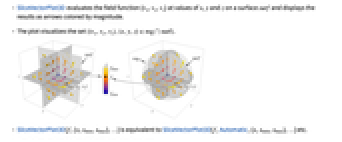
- SliceVectorPlot3D evaluates the field function {vx,vy,vz} at values of x, y and z on a surface surf and displays the results as arrows colored by magnitude.
- The plot visualizes the set
 .
. - SliceVectorPlot3D[f,{x,xmin,xmax},…] is equivalent to SliceVectorPlot3D[f,Automatic,{x,xmin,xmax},…] etc.
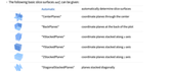
- The following basic slice surfaces surfi can be given:
-
Automatic automatically determine slice surfaces 
"CenterPlanes" coordinate planes through the center 
"BackPlanes" coordinate planes at the back of the plot 
"XStackedPlanes" coordinate planes stacked along  axis
axis
"YStackedPlanes" coordinate planes stacked along  axis
axis
"ZStackedPlanes" coordinate planes stacked along  axis
axis
"DiagonalStackedPlanes" planes stacked diagonally 
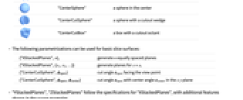
"CenterSphere" a sphere in the center 
"CenterCutSphere" a sphere with a cutout wedge 
"CenterCutBox" a box with a cutout octant - The following parametrizations can be used for basic slice surfaces:
-
{"XStackedPlanes",n}, generate n equally spaced planes {"XStackedPlanes",{x1,x2,…}} generate planes for x=xi {"CenterCutSphere",ϕopen} cut angle ϕopen facing the view point {"CenterCutSphere",ϕopen,ϕcenter} cut angle ϕopen with center angle ϕcenter in the  plane
plane - "YStackedPlanes", "ZStackedPlanes" follow the specifications for "XStackedPlanes", with additional features shown in the scope examples.
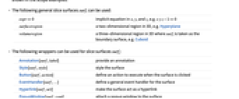
- The following general slice surfaces surfi can be used:
-
expr0 implicit equation in x, y, and z, e.g. x y z-10 surfaceregion a two-dimensional region in 3D, e.g. Hyperplane volumeregion a three-dimensional region in 3D where surfi is taken as the boundary surface, e.g. Cuboid - The following wrappers can be used for slice surfaces surfi:
-
Annotation[surf,label] provide an annotation Style[surf,style] style the surface Button[surf,action] define an action to execute when the surface is clicked EventHandler[surf,…] define a general event handler for the surface Hyperlink[surf,uri] make the surface act as a hyperlink PopupWindow[surf,cont] attach a popup window to the surface StatusArea[surf,label] display in status area when the surface is moused over Tooltip[surf,label] attach an arbitrary tooltip to the surface - SliceVectorPlot3D has the same options as Graphics3D, with the following additions and changes: [List of all options]
-
Axes True whether to draw axes BoundaryStyle Automatic how to style surface boundaries BoxRatios {1,1,1} ratio of height to width ClippingStyle Automatic how to display arrows outside the vector range Method Automatic methods to use for the plot PerformanceGoal $PerformanceGoal aspects of performance to try to optimize PlotLegends None legends to include PlotPoints Automatic approximate number of samples for the slice surfaces surfi in each direction PlotRange {Full,Full,Full} range of x, y, z values to include PlotRangePadding Automatic how much to pad the range of values PlotStyle Automatic style directives for each slice surface PlotTheme $PlotTheme overall theme for the plot RegionBoundaryStyle None how to style plot region boundaries RegionFunction (True&) determine what region to include ScalingFunctions None how to scale axes TargetUnits Automatic desired units to use VectorAspectRatio Automatic width-to-length ratio for arrows VectorColorFunction Automatic how to color vectors VectorColorFunctionScaling True whether to scale the argument to VectorColorFunction VectorMarkers Automatic the shape of the arrows VectorPoints Automatic the number or placement of vectors to plot VectorRange Automatic range of vector lengths to show VectorScaling None how to scale the sizes of arrows VectorSizes Automatic sizes of displayed arrows VectorStyle Automatic how to draw vectors WorkingPrecision MachinePrecision precision to use in internal computations - VectorScaling scales the magnitudes of the vectors into the range of arrow sizes smin to smax given by VectorSizes.
- VectorScaling->Automatic will scale the arrow lengths depending on the vector magnitudes:
- RegionFunction is supplied with x, y, z, vx, vy, vz, Norm[{vx,vy,vz}].
- VectorColorFunction is by default supplied with scaled x, y, z, vx, vy, vz, Norm[{vx,vy,vz}].
- Slice surfaces can be styled using a Style wrapper and PlotStyle option, with the Style wrapper taking precedence over PlotStyle. None can be used to indicate that no slice surface should be shown.
- Possible settings for ScalingFunctions include:
-
{sx,sy,sz} scale x, y and z axes - Common built-in scaling functions s include:
-
"Log" 
log scale with automatic tick labeling "Log10" 
base-10 log scale with powers of 10 for ticks "SignedLog" 
log-like scale that includes 0 and negative numbers "Reverse" 
reverse the coordinate direction "Infinite" 
infinite scale -
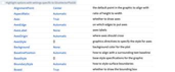
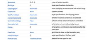
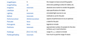
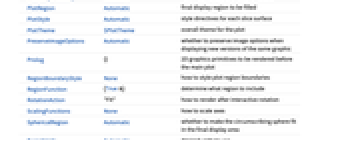
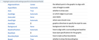
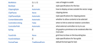
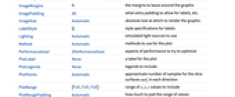
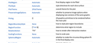
AlignmentPoint Center the default point in the graphic to align with AspectRatio Automatic ratio of height to width Axes True whether to draw axes AxesEdge Automatic on which edges to put axes AxesLabel None axes labels AxesOrigin Automatic where axes should cross AxesStyle {} graphics directives to specify the style for axes Background None background color for the plot BaselinePosition Automatic how to align with a surrounding text baseline BaseStyle {} base style specifications for the graphic BoundaryStyle Automatic how to style surface boundaries Boxed True whether to draw the bounding box BoxRatios {1,1,1} ratio of height to width BoxStyle {} style specifications for the box ClippingStyle Automatic how to display arrows outside the vector range ClipPlanes None clipping planes ClipPlanesStyle Automatic style specifications for clipping planes ContentSelectable Automatic whether to allow contents to be selected ControllerLinking False when to link to external rotation controllers ControllerPath Automatic what external controllers to try to use Epilog {} 2D graphics primitives to be rendered after the main plot FaceGrids None grid lines to draw on the bounding box FaceGridsStyle {} style specifications for face grids FormatType TraditionalForm default format type for text ImageMargins 0. the margins to leave around the graphic ImagePadding All what extra padding to allow for labels, etc. ImageSize Automatic absolute size at which to render the graphic LabelStyle {} style specifications for labels Lighting Automatic simulated light sources to use Method Automatic methods to use for the plot PerformanceGoal $PerformanceGoal aspects of performance to try to optimize PlotLabel None a label for the plot PlotLegends None legends to include PlotPoints Automatic approximate number of samples for the slice surfaces surfi in each direction PlotRange {Full,Full,Full} range of x, y, z values to include PlotRangePadding Automatic how much to pad the range of values PlotRegion Automatic final display region to be filled PlotStyle Automatic style directives for each slice surface PlotTheme $PlotTheme overall theme for the plot PreserveImageOptions Automatic whether to preserve image options when displaying new versions of the same graphic Prolog {} 2D graphics primitives to be rendered before the main plot RegionBoundaryStyle None how to style plot region boundaries RegionFunction (True&) determine what region to include RotationAction "Fit" how to render after interactive rotation ScalingFunctions None how to scale axes SphericalRegion Automatic whether to make the circumscribing sphere fit in the final display area TargetUnits Automatic desired units to use Ticks Automatic specification for ticks TicksStyle {} style specification for ticks TouchscreenAutoZoom False whether to zoom to fullscreen when activated on a touchscreen VectorAspectRatio Automatic width-to-length ratio for arrows VectorColorFunction Automatic how to color vectors VectorColorFunctionScaling True whether to scale the argument to VectorColorFunction VectorMarkers Automatic the shape of the arrows VectorPoints Automatic the number or placement of vectors to plot VectorRange Automatic range of vector lengths to show VectorScaling None how to scale the sizes of arrows VectorSizes Automatic sizes of displayed arrows VectorStyle Automatic how to draw vectors ViewAngle Automatic angle of the field of view ViewCenter Automatic point to display at the center ViewMatrix Automatic explicit transformation matrix ViewPoint {1.3,-2.4,2.} viewing position ViewProjection Automatic projection method for rendering objects distant from the viewer ViewRange All range of viewing distances to include ViewVector Automatic position and direction of a simulated camera ViewVertical {0,0,1} direction to make vertical WorkingPrecision MachinePrecision precision to use in internal computations
List of all options
Examples
open all close allScope (28)
Surfaces (9)
Generate a plot over standard slice surfaces:
Standard axis-aligned stacked slice surfaces:
Plotting over a volume primitive is equivalent to plotting over RegionBoundary[reg]:
Plot a vector field over multiple slice surfaces:
Sampling (3)
Use VectorPoints to specify the number of arrows:
Use RegionFunction to expose obscured slices:
The domain may be specified by a region including Cone:
A formula region including ImplicitRegion:
A mesh-based region including BoundaryMeshRegion:
Presentation (16)
Use VectorScaling to show arrows scaled according to their magnitudes:
Use VectorSizes to prevent arrows from being too small:
Use VectorRange to control which vectors are plotted:
Use ClippingStyle to control the appearance of the clipped vectors:
Use PlotTheme to immediately get overall styling:
Use PlotLegends to get a color bar for the different values:
Control the display of axes with Axes:
Label axes using AxesLabel and the whole plot using PlotLabel:
Color the vectors by their magnitude with VectorColorFunction:
Use VectorMarkers to control the shape of the vectors:
Use VectorAspectRatio to modify the width-to-length ratio of the arrows:
Style the slice surface boundaries with BoundaryStyle:
Highlight a RegionFunction with RegionBoundaryStyle:
Style a RegionFunction with RegionBoundaryStyle:
TargetUnits specifies which units to use in the visualization:
Options (88)
Axes (3)
AxesLabel (4)
No axes labels are drawn by default:
Use specific labels for each axis:
Use labels based on variables specified in SliceVectorPlot3D:
AxesOrigin (2)
AxesStyle (3)
BoxRatios (3)
ClippingStyle (4)
By default, clipped vectors are given a constant color that is consistent with the minimum or maximum vector lengths given by VectorRange:
ImageSize (7)
Use named sizes such as Tiny, Small, Medium and Large:
Specify the width of the plot:
Specify the height of the plot:
Allow the width and height to be up to a certain size:
Specify the width and height for a graphic, padding with space if necessary:
Setting AspectRatioFull will fill the available space:
Use maximum sizes for the width and height:
Use ImageSizeFull to fill the available space in an object:
Specify the image size as a fraction of the available space:
PerformanceGoal (2)
PlotLegends (3)
No legends are included by default:
Include a legend that indicates the vector norms by color:
With multiple fields and VectorColorFunction set to None, use a legend to identify each field:
PlotRange (2)
PlotRangePadding (7)
PlotTheme (3)
Override PlotTheme styles by explicitly setting options:
RegionBoundaryStyle (3)
By default, a region function is not explicitly shown:
A similar effect can be created by combining VectorRange and ClippingStyle:
RegionFunction (3)
ScalingFunctions (4)
Ticks (6)
Ticks are placed automatically in each plot:
Use TicksNone to not draw any tick marks:
Place tick marks at specific positions:
Draw tick marks at the specified positions with the specified labels:
Specify tick marks with scaled lengths:
Customize each tick with position, length, labeling and styling:
TicksStyle (3)
VectorAspectRatio (1)
VectorAspectRatio specifies the width of the arrow over its length:
VectorColorFunction (5)
By default, vectors are colored according to their norm:
Use any named color gradient from ColorData:
Color the vectors according to their ![]() value:
value:
Use VectorColorFunctionScaling->False to get unscaled values:
VectorColorFunctionScaling (3)
By default, scaled values are used:
Use VectorColorFunctionScaling->False to get unscaled values:
Explicitly specify the scaling for each color function argument:
VectorMarkers (3)
The default vector marker is "Arrow3D":
By default, arrows are centered at sampled points. Use Placed to start the arrow at the sampled point:
VectorPoints (4)
VectorRange (3)
Specify the range of vector norms that are displayed with varying color:
Combine with ClippingStyle to remove the clipped vectors:
VectorScaling (3)
By default, arrows are displayed with a constant length:
Use Automatic to scale arrows proportionally to the corresponding vector norm:
Use VectorSizes to specify the range of relative lengths of the arrows:
VectorSizes (2)
Make the vectors half of the default size:
With VectorScaling, VectorSizes controls the range of the lengths of the arrows relative to the default size:
VectorStyle (1)
VectorColorFunction has precedence over VectorStyle:
Applications (23)
Basic Vector Fields (3)
Differential Equations (9)
Illustrate the behavior of a linear system of differential equations ![]() in the case when
in the case when ![]() is diagonal:
is diagonal:
Solve the corresponding differential equation starting on the slice surfaces:
The differential equation solution follows the arrows in the plot all converging to the origin:
Automate the previous example and analyze all the possible sign combinations of the real eigenvalues for ![]() , where
, where ![]() is a diagonal matrix with eigenvalues
is a diagonal matrix with eigenvalues ![]() :
:
For ![]() , there is stability along the
, there is stability along the ![]() ,
, ![]() , and
, and ![]() directions:
directions:
For ![]() , there is stability along
, there is stability along ![]() and
and ![]() , but instability along
, but instability along ![]() :
:
For ![]() , there is stability along
, there is stability along ![]() and instability along
and instability along ![]() and
and ![]() :
:
For ![]() , there is instability along
, there is instability along ![]() ,
, ![]() , and
, and ![]() :
:
Define a matrix ![]() and compute its eigenvalues:
and compute its eigenvalues:
Since ![]() is symmetric, its eigenspaces
is symmetric, its eigenspaces ![]() ,
, ![]() and
and ![]() are mutually orthogonal:
are mutually orthogonal:
Generate the orthogonal complements of the eigenspaces:
Plot the vector field ![]() and observe the effects of the eigenvalues:
and observe the effects of the eigenvalues:
The plane orthogonal to ![]() contains
contains ![]() and
and ![]() , so the origin is attractive in
, so the origin is attractive in ![]() and repulsive in
and repulsive in ![]() :
:
The plane orthogonal to ![]() contains
contains ![]() and
and ![]() , so the field points directly toward
, so the field points directly toward ![]() :
:
The plane orthogonal to ![]() contains
contains ![]() and
and ![]() , so the field points directly away from
, so the field points directly away from ![]() :
:
Define a matrix ![]() and compute its eigenvalues:
and compute its eigenvalues:
The eigenvalues and eigenvectors of ![]() indicate a sink at the origin for the vector field
indicate a sink at the origin for the vector field ![]() with spiral behavior around the
with spiral behavior around the ![]() axis:
axis:
Examine the vector field ![]() in planes orthogonal to
in planes orthogonal to ![]() :
:
Compute solutions of the linear system of differential equations ![]() for several initial conditions:
for several initial conditions:
Add the solutions of ![]() to the vector field:
to the vector field:
Define a new matrix ![]() and compute its eigenvalues and eigenvectors:
and compute its eigenvalues and eigenvectors:
The eigenspace ![]() is a plane through the origin with normal
is a plane through the origin with normal ![]() , so solutions of
, so solutions of ![]() are attracted to the origin while spiraling around
are attracted to the origin while spiraling around ![]() :
:
Illustrate the behavior of a linear system of differential equations ![]() in the case when
in the case when ![]() is block diagonal, with one real and two complex conjugate eigenvalues. The matrix
is block diagonal, with one real and two complex conjugate eigenvalues. The matrix  has eigenvalues
 ![]() ,
, ![]() , and
, and ![]() :
:
Construct a matrix ![]() with eigenvalues
with eigenvalues ![]() ,
, ![]() , and
, and ![]() :
:
Find solutions to the corresponding differential equation:
Show vector field and solutions together:
Automate the previous example and analyze for different real ![]() and
and ![]() :
:
Solve an initial value problem with a solution that is contained in a cylinder:
Graph the surface, the vector field on the surface and the solution of the initial value problem:
Solve an initial value problem with a solution contained in a sphere:
Graph the surface, the vector field on the surface and the solution of the initial value problem:
Solve an initial value problem with a solution contained in a hyperbolic paraboloid:
Graph the surface, the vector field on the surface and the solution of the initial value problem:
Fluid Dynamics (2)
Solid Mechanics (2)
A solid cylinder with a tensile load:
A solid cylinder with a compressive load:
A hollow cylinder with internal and external pressures:
An elastic bar in the shape of a circular cylinder with radius 1 has a net torque ![]() applied at both ends. The resulting displacement field is
applied at both ends. The resulting displacement field is ![]() , where
, where ![]() is the shear modulus, the nonzero stresses are
is the shear modulus, the nonzero stresses are ![]() and
and ![]() and the forces on the surfaces
and the forces on the surfaces ![]() are the tractions:
are the tractions:
Display the displacement field that results from the applied forces:
Electromagnetism (1)
Flux (3)
Visualize the outward pointing unit normal vectors to a surface:
Define vector field ![]() and compute the unit normals to the surface
and compute the unit normals to the surface ![]() :
:
Visualize the vector field ![]() and the unit normals to
and the unit normals to ![]() :
:
The flux density of ![]() through
through ![]() is zero since
is zero since ![]() is orthogonal to the normals of
is orthogonal to the normals of ![]() :
:
Define vector field ![]() and compute the unit normals to the surface
and compute the unit normals to the surface ![]() :
:
Visualize the vector field ![]() and the unit normals to
and the unit normals to ![]() :
:
Compute the flux density of ![]() through
through ![]() :
:
The total flux is zero because the negative flux is canceled by the positive flux. Visualize this by coloring the surface by the flux density:
Other Applications (3)
Visualize the "hairy ball theorem" (https://mathworld.wolfram.com/HairyBallTheorem.html) that, loosely speaking, says that you cannot comb the hair on a sphere without leaving a whorl:
Show a vector field in a tangent plane:
Choose 10 random points on the unit sphere:
Compute the angles ϕ and θ for the points at ![]() :
:
Plot geodesics from ![]() to the target points:
to the target points:
Show the sphere, geodesics, target points, and a vector field of tangents for the geodesics:
Properties & Relations (10)
Use VectorPlot3D for a full volume visualization of the vector field:
Use ListSliceVectorPlot3D for data:
Use VectorPlot for vector plots in 2D:
Use StreamPlot or LineIntegralConvolutionPlot for vector fields in 2D:
Use VectorDensityPlot to add a density plot of a scalar field:
Use StreamDensityPlot to use streams instead of vectors:
Use VectorDisplacementPlot to visualize the effect of a displacement vector field on a specified region:
Use VectorDisplacementPlot3D to visualize the effect of a displacement vector field on a specified 3D region:
Use StreamPlot3D to plot 3D fields as streamlines:
Plot complex functions as a vector field with ComplexVectorPlot:
Plot streams instead of vectors with ComplexStreamPlot:
Use GeoVectorPlot to plot vectors on a map:
Use GeoStreamPlot to use streams instead of vectors:
Text
Wolfram Research (2015), SliceVectorPlot3D, Wolfram Language function, https://reference.wolfram.com/language/ref/SliceVectorPlot3D.html (updated 2022).
CMS
Wolfram Language. 2015. "SliceVectorPlot3D." Wolfram Language & System Documentation Center. Wolfram Research. Last Modified 2022. https://reference.wolfram.com/language/ref/SliceVectorPlot3D.html.
APA
Wolfram Language. (2015). SliceVectorPlot3D. Wolfram Language & System Documentation Center. Retrieved from https://reference.wolfram.com/language/ref/SliceVectorPlot3D.html