BodePlot
詳細とオプション
- BodePlotは lsys の伝達関数のゲインと位相の線図を与える.
- 系 lsys はディスクリプタ系と遅延系を含むTransferFunctionModelまたはStateSpaceModelである.
- 対応する伝達関数
がある系 lsys に対しては,次の式の線図が与えられる. -

連続時間系 

サンプル時間
の離散時間系 - BodePlotは,事実上Blockを使い,変数 ω を局所的なものとして扱う.
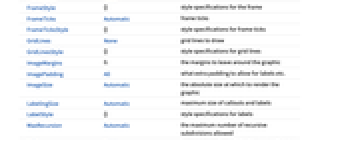
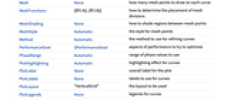
- BodePlotにはPlotと同じオプションに以下の追加・変更を加えたものが使える. [全オプションのリスト]
-
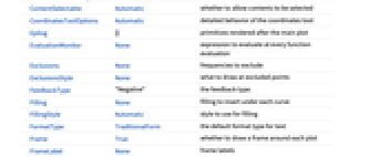
Exclusions None 除外する周波数 FeedbackType "Negative" フィードバックタイプ Frame True 各プロットに枠を描くかどうか MeshFunctions {{#1&},{#1&}} メッシュ区分の置き方の決め方 PhaseRange Automatic 使用する位相値の範囲 PlotLayout "VerticalGrid" 使用するレイアウト PlotRange {{Full,Automatic},{Full,Automatic}} 含める値の範囲 SamplingPeriod None サンプリング周期 ScalingFunctions {{"Log10","dB"},{"Log10","Degree"}} スケーリング関数 StabilityMargins False 安定余裕を示すかどうか StabilityMarginsStyle Automatic 安定余裕のスタイルを指定するグラフィックス指示子 - ColorData["DefaultPlotColors"]は,PlotStyleで使われるデフォルトの色のシーケンスを与える.
- オプションPlotLayoutで使える明示的な設定値は"VerticalGrid"と"List"である.
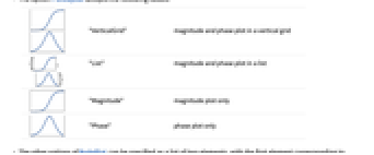
- オプションPlotLayoutには次の値が使える.
-
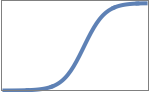
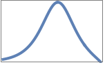
"VerticalGrid" ゲイン線図と位相線図を垂直格子で {
,
}"List" ゲイン線図と位相線図をリストで 
"Magnitude" ゲイン線図のみ 
"Phase" 位相線図のみ - BodePlotの他のオプションは,最初の要素がゲイン線図,2番目が位相線図を表す,2つの要素のリストとして指定できる.
- オプション指定
-
opt->val val をゲインと位相の両線図に使う opt->{val} val をゲイン線図に,デフォルト値を位相線図に使う opt->{val1,val2} val1をゲイン線図に,val2を位相線図に使う opt->{Automatic,val} デフォルト値をゲイン線図に,val を位相線図に使う - PlotLayoutの設定が"Magnitude"あるいは"Phase"のとき,単一の設定は要求された線図を参照する.
- スケーリング関数はScalingFunctions{{magfreqscale,magscale},{phasefreqscale,phasescale}}で指定できる.
- 周波数スケール magfreqscale と phasefreqscale には,10を底とする対数スケールを表す"Log10"と線形スケールを表す"Linear"が使える.
- ゲインスケール magscale にはそれぞれゲインのデシベルと絶対値を表す"dB"あるいは"Absolute"が使える.
- 位相スケール phasescale には"Degree"あるいは"Radian"が使える.
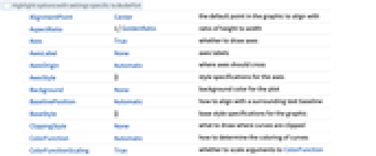
全オプションのリスト
例題
すべて開く すべて閉じる例 (3)
BodePlot[TransferFunctionModel[{{{20}}, 20 + s}, s]]lsys[ω_, ζ_] := TransferFunctionModel[{{{ω^2}}, s^2 +
2*s*ζ*ω + ω^2}, s];BodePlot[lsys[1, 1], {.01, 100}]BodePlot[StateSpaceModel[{{{0, 1}, {-0.5, -0.05}}, {{0}, {1}}, {{1, 0}}, {{0}}}, SamplingPeriod -> None,
SystemsModelLabels -> None]]スコープ (13)
BodePlot[TransferFunctionModel[{{{10}}, 1}, s]]BodePlot[TransferFunctionModel[{{{1}}, s}, s]]BodePlot[TransferFunctionModel[{{{s}}, 1}, s]]BodePlot[TransferFunctionModel[{{{1}}, 1 + 10*s}, s]]BodePlot[TransferFunctionModel[{{{1 + 10*s}}, 1}, s]]BodePlot[TransferFunctionModel[{{{100}}, 100 + 1.*s + s^2}, s]]BodePlot[TransferFunctionModel[{{{5*(1 + 0.1*s)}}, s + 0.512*s^2 +
0.0064*s^3 + 0.0002*s^4}, s]]BodePlot[TransferFunctionModel[{{{E^(-0.5*s)}}, 1. + 2.*s}, s]]BodePlot[TransferFunctionModel[{{{-0.9 + z}}, -0.8 + z}, z,
SamplingPeriod -> 1]]BodePlot[TransferFunctionModel[{{{-4 + 4.9*z}}, (-4.5 + z)*(-1 + z)},
z, SamplingPeriod -> 1], {0.05, (π/2)}]BodePlot[StateSpaceModel[{{{-1, 10, 0}, {-2, -7, 335}, {0, 0, -10}}, {{0}, {0}, {10}}, {{1, 0, 0}}, {{0}}},
SamplingPeriod -> None, SystemsModelLabels -> None]]BodePlot[(10/20ω I + 1), {ω, 0.0005, 10}]BodePlot[TransferFunctionModel[{{{2, 1}, {0.5, 0.1}}, {{1 + s, 2 + s},
{3 + s, 4 + s}}}, s]]一般化と拡張 (1)
オプション (21)
CoordinatesToolOptions (5)
BodePlot[TransferFunctionModel[{{{2500}}, 15500 + 400*s + s^2}, s]]周波数rad/sであるなら,これを
で割って座標周波数の値をHzで得る:
BodePlot[TransferFunctionModel[{{{4}}, 4 + 2*s + s^2}, s], CoordinatesToolOptions -> ("DisplayFunction" -> Function[pt, {(pt[[1]]/2 π), pt[[2]]}])]BodePlot[TransferFunctionModel[{{{16}}, (1 + s)*(4 + s)^2}, s], CoordinatesToolOptions -> {"DisplayFunction" -> Function[pt, {(pt[[1]]/2 π), pt[[2]]}]}]もとの単位による周波数値,絶対単位によるゲイン,ラジアンによる位相:
BodePlot[TransferFunctionModel[{{{5}}, s*(10 + 6*s + s^2)},
s], CoordinatesToolOptions -> {{"DisplayFunction" -> Function[pt, {pt[[1]], 10^(pt[[2]]/20)}]}, {"DisplayFunction" -> Function[pt, {pt[[1]], pt[[2]] Degree}]}}]BodePlot[TransferFunctionModel[{{{100*s}}, 1 + s}, s], CoordinatesToolOptions -> {Automatic, {"DisplayFunction" -> Function[pt, {pt[[1]], pt[[2]] Degree}], "CopiedValueFunction" -> Function[pt, {pt[[1]], pt[[2]]Degree}]}}]GridLines (3)
BodePlot[TransferFunctionModel[{{{1.6}}, 1.6 + 3*s + s^2}, s], GridLines -> Automatic]BodePlot[TransferFunctionModel[{{{10}}, (2 + s)*(4 + s)*(6 + s)},
s], GridLines -> {Automatic, None}]BodePlot[TransferFunctionModel[{{{1}}, s^2*(3 + s + s^2)},
s], GridLines -> {{List[0.01, 0.1, 1, 10], Range[-150, 140, 20]}, {List[0.01, 0.1, 1, 10], Range[0, 200, 25]}}]GridLinesStyle (2)
BodePlot[TransferFunctionModel[{{{1}}, 10 + 3*s + s^3}, s], GridLines -> Automatic, GridLinesStyle -> Red]BodePlot[TransferFunctionModel[{{{1 + s}}, s*(2 + s)*
(3 + s)}, s], GridLines -> Automatic, GridLinesStyle -> {{Green, Orange}, {Red, Orange}}]PhaseRange (1)
PlotLayout (1)
tfm = TransferFunctionModel[{{{-5 + s}},
s*(1 + 3*s + s^2)}, s];BodePlot[tfm, PlotLabel -> {"Magnitude Plot", "Phase Plot"}]BodePlot[tfm, PlotLayout -> "list", PlotLabel -> {"magnitude", "phase"}]BodePlot[tfm, PlotLayout -> "Magnitude"]BodePlot[tfm, PlotLayout -> "Phase"]PlotTheme (2)
SamplingPeriod (2)
tfm = TransferFunctionModel[{{{0.5}}, (-0.1 + z)*z^2}, z,
SamplingPeriod -> 1];BodePlot[tfm, {0.1, Pi}]BodePlot関数でサンプリング周期を指定する:
BodePlot[(5/(-0.1 + z) z^2), {0.1, π}, SamplingPeriod -> 1]BodePlot[(5/(-0.1 + z) z^2), {0.1, π}, SamplingPeriod -> 0.5]ScalingFunctions (2)
BodePlot[TransferFunctionModel[{{{1}}, (1 + s)*(1 + 10*s)}, s], {0.1, 10}, ScalingFunctions -> {{Automatic, "Absolute"}, {Automatic, "Radian"}}]BodePlot[TransferFunctionModel[{{{1 + s}}, 1 + 5*s + s^2},
s], {0.1, 10}, ScalingFunctions -> {{"Linear", Automatic}, {"Linear", Automatic}}]StabilityMargins (2)
アプリケーション (7)
タイプ0系の静止位置誤差定数は定常状態におけるゲインである:
BodePlot[TransferFunctionModel[{{{10}}, 1 + s}, s], {0.001, 10}, Epilog -> {PointSize[Medium], Red, Point[{Log10[0.001], 20 Log10[Limit[(10/s + 1), s -> 0]]}]}, PlotRange -> {{0.0008, 10}, Automatic}, PlotLayout -> "Magnitude", Frame -> False]BodePlot[ TransferFunctionModel[{{{z}}, (-0.6 + z)*(-0.05 + z)},
z, SamplingPeriod -> 0.5], {0.001, (π/0.5)}, Epilog -> {PointSize[Medium], Red, Point[{Log10[0.001], 20 Log10[Limit[(z/(z - 0.05) (z - 0.6)), z -> 1]]}]}, PlotRange -> {{0.0008, (π/0.5)}, Automatic}, PlotLayout -> "Magnitude", Frame -> False]タイプ1系の静止速度誤差定数は0 dBラインと最初の10年における
デシベルのセグメント(あるいはその延長)のほぼ交点である:
BodePlot[TransferFunctionModel[{{{5}}, s*(3 + s)}, s], {0.1, 100}, Epilog -> {Line[{{Log10[0.1], 0}, {Log10[100], 0}}], PointSize[Large], Red, Point[{ Log10[Limit[s (5 /s(s + 3)), s -> 0]], 0}]}, PlotLayout -> "Magnitude", Frame -> False]BodePlot[TransferFunctionModel[{{{1}}, (-1 + z)*(-0.025 + z)}, z,
SamplingPeriod -> 1], {0.1, π}, Epilog -> {Line[{{Log10[0.1], 0}, {Log10[π], 0}}], PointSize[Medium], Red, Point[{Log10[Limit[(z - 1/(z - 1) (z - 0.025)), z -> 1]], 0}]}, PlotLayout -> "Magnitude", Frame -> False]タイプ2の系の静止加速度誤差定数の平方根は最初の10年間に
デシベルのセグメント(あるいはその延長)と0 dB線とのほぼ交点である:
BodePlot[TransferFunctionModel[{{{1}}, s^2*(1 + s)}, s], {0.1, 10}, Epilog -> {Line[{{Log10[0.1], 0}, {Log10[10], 0}}], PointSize[Medium], Red, Point[{ Log10[Sqrt[Limit[s^2(1/s^2(s + 1)), s -> 0]]], 0}]}, PlotLayout -> "Magnitude", Frame -> False]BodePlot[TransferFunctionModel[{{{0.0001*z}}, (-1 + z)^2*
(0.1 - 0.3*z + z^2)}, z, SamplingPeriod -> 1], {0.001, π}, Epilog -> {Line[{{Log10[0.001], 0}, {Log10[π], 0}}], PointSize[Medium], Red, Point[{Log10[Sqrt[Limit[((z - 1)^2 (0.0001 z)/(z - 1)^2 (z^2 - 0.3 z + 0.1)), z -> 1]]], 0}]}, PlotLayout -> "Magnitude", Frame -> False]BodePlot[{Tooltip[TransferFunctionModel[{{{583900}}, s*(36 + s)*(100 + s)},
s]], Tooltip[TransferFunctionModel[{{{36786*(0.98 + s)}}, s*(0.062 + s)*
(36 + s)*(100 + s)}, s]]}, StabilityMargins -> {True, True}, StabilityMarginsStyle -> {RGBColor[0.24, 0.6, 0.8], RGBColor[0.95, 0.627, 0.1425]}, PlotStyle -> {RGBColor[0.24, 0.6, 0.8], RGBColor[0.95, 0.627, 0.1425]}, PlotLayout -> "Phase", Frame -> False]サンプリング周期が1のゼロ次ホールドの周波数応答を可視化する:
BodePlot[TransferFunctionModel[{{{(-1 + E^s)/E^s}}, s},
s], {0.01, 30}, ScalingFunctions -> {{"Linear", "Absolute"}, {"Linear", "Degree"}}, PlotRange -> All]ラプラス変数がラジアン/秒のときに,周波数がヘルツのボード線図を得る:
tfm = TransferFunctionModel[{{{100}}, s*(100 + 10*s + s^2)},
s];BodePlot[tfm[I 2 π f], f]連続時間系については,ラプラス変数をスケールすることで,同じ結果を得ることができる:
BodePlot[tfm[2 π s]]ラジアン/秒のZ変換変数による離散時間系についてのヘルツの点:
BodePlot[(-0.4 + E^2 I f π/0.5 + E^2 I f π), f, SamplingPeriod -> 1]特性と関係 (1)
SingularValuePlotはボード線図のゲイン線図を多入力多出力系に一般化する:
tfm = TransferFunctionModel[{{{10000}}, (5 + s)*(20 + s)*
(50 + s)}, s];{SingularValuePlot[tfm], BodePlot[tfm, PlotLayout -> "Magnitude", Frame -> False]}関連するガイド
-
▪
- 古典制御理論と設計 ▪
- フーリエ(Fourier)解析 ▪
- 積分変換 ▪
- 制御系 ▪
- 信号フィルタリングとフィルタ設計 ▪
- 総和変換 ▪
- 遅延制御系 ▪
- システムモデルの解析と設計
テキスト
Wolfram Research (2010), BodePlot, Wolfram言語関数, https://reference.wolfram.com/language/ref/BodePlot.html (2014年に更新).
CMS
Wolfram Language. 2010. "BodePlot." Wolfram Language & System Documentation Center. Wolfram Research. Last Modified 2014. https://reference.wolfram.com/language/ref/BodePlot.html.
APA
Wolfram Language. (2010). BodePlot. Wolfram Language & System Documentation Center. Retrieved from https://reference.wolfram.com/language/ref/BodePlot.html
BibTeX
@misc{reference.wolfram_2026_bodeplot, author="Wolfram Research", title="{BodePlot}", year="2014", howpublished="\url{https://reference.wolfram.com/language/ref/BodePlot.html}", note=[Accessed: 10-August-2026]}
BibLaTeX
@online{reference.wolfram_2026_bodeplot, organization={Wolfram Research}, title={BodePlot}, year={2014}, url={https://reference.wolfram.com/language/ref/BodePlot.html}, note=[Accessed: 10-August-2026]}