BodePlot
更多信息和选项
- BodePlot 绘制 lsys 的传递函数的幅值和相位.
- 系统 lsys 可以是 TransferFunctionModel 或者 StateSpaceModel,包含描述器或者延迟系统.
- 对于相应的传递函数为
的系统 lsys,可以绘制下列表达式的图线: -

连续时间系统 
采样时间
下的离散时间系统 - BodePlot 将变量 ω 视为局部变量,使用 Block.
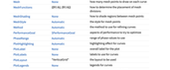
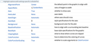
- BodePlot 具有与 Plot 相同的选项,并具有以下变化和增加: [所有选项的列表]
-
Exclusions None 要排除的频率 FeedbackType "Negative" 反馈类型 Frame True 是否在每个图线周围绘制框 MeshFunctions {{#1&},{#1&}} 如何决定网格划分的位置 PhaseRange Automatic 要使用的相位值范围 PlotLayout "VerticalGrid" 要使用的布局 PlotRange {{Full,Automatic},{Full,Automatic}} 要包括的值的范围 SamplingPeriod None 采样周期 ScalingFunctions {{"Log10","dB"},{"Log10","Degree"}} 尺度函数 StabilityMargins False 是否显示稳定裕度 StabilityMarginsStyle Automatic 指定稳定裕度样式的图形指令 - ColorData["DefaultPlotColors"] 给出 PlotStyle 使用的默认颜色序列.
- 选项 PlotLayout 的可能明确设置是 "VerticalGrid" 和 "List".
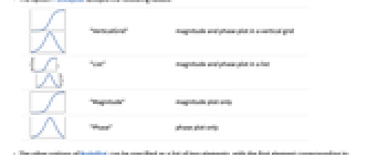
- 选项 PlotLayout 接受下列值:
-
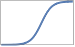
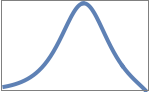
"VerticalGrid" 在垂直网格上的幅值和相位图 {
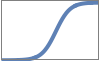
,
}"List" 列表中的幅值和相位图 
"Magnitude" 仅幅值图 
"Phase" 仅相位图 - BodePlot 的其它选项可用二元素列表指定,其中第一个元素对应于幅值图形,第二个元素对应于相位图形.
- 选项的指定包括:
-
opt->val 幅值与相位图均使用 val opt->{val} 幅值图使用 val,相位图使用默认值 opt->{val1,val2} 幅值图使用 val1,相位图使用 val2 opt->{Automatic,val} 幅值图使用默认值,相位图使用 val - 在 PlotLayout 的设置为 "Magnitude" 或 "Phase" 时,一个单一设置指向所要求的图形.
- 尺度函数可由 ScalingFunctions->{{magfreqscale,magscale},{phasefreqscale,phasescale}} 指定.
- 频率尺度 magfreqscale 与 phasefreqscale 可以为 "Log10" 或 "Linear",这分别对应于以10为基底的对数尺度和线性尺度.
- 幅度尺度 magscale 可以是 "dB" 或者 "Absolute",它们分别对应于幅度的十进制和绝对值.
- 相位尺度 phasescale 可以是 "Degree" 或者 "Radian".
所有选项的列表
范例
打开所有单元 关闭所有单元基本范例 (3)
BodePlot[TransferFunctionModel[{{{20}}, 20 + s}, s]]lsys[ω_, ζ_] := TransferFunctionModel[{{{ω^2}}, s^2 +
2*s*ζ*ω + ω^2}, s];BodePlot[lsys[1, 1], {.01, 100}]BodePlot[StateSpaceModel[{{{0, 1}, {-0.5, -0.05}}, {{0}, {1}}, {{1, 0}}, {{0}}}, SamplingPeriod -> None,
SystemsModelLabels -> None]]范围 (13)
BodePlot[TransferFunctionModel[{{{10}}, 1}, s]]BodePlot[TransferFunctionModel[{{{1}}, s}, s]]BodePlot[TransferFunctionModel[{{{s}}, 1}, s]]BodePlot[TransferFunctionModel[{{{1}}, 1 + 10*s}, s]]BodePlot[TransferFunctionModel[{{{1 + 10*s}}, 1}, s]]BodePlot[TransferFunctionModel[{{{100}}, 100 + 1.*s + s^2}, s]]BodePlot[TransferFunctionModel[{{{5*(1 + 0.1*s)}}, s + 0.512*s^2 +
0.0064*s^3 + 0.0002*s^4}, s]]BodePlot[TransferFunctionModel[{{{E^(-0.5*s)}}, 1. + 2.*s}, s]]BodePlot[TransferFunctionModel[{{{-0.9 + z}}, -0.8 + z}, z,
SamplingPeriod -> 1]]BodePlot[TransferFunctionModel[{{{-4 + 4.9*z}}, (-4.5 + z)*(-1 + z)},
z, SamplingPeriod -> 1], {0.05, (π/2)}]BodePlot[StateSpaceModel[{{{-1, 10, 0}, {-2, -7, 335}, {0, 0, -10}}, {{0}, {0}, {10}}, {{1, 0, 0}}, {{0}}},
SamplingPeriod -> None, SystemsModelLabels -> None]]BodePlot[(10/20ω I + 1), {ω, 0.0005, 10}]BodePlot[TransferFunctionModel[{{{2, 1}, {0.5, 0.1}}, {{1 + s, 2 + s},
{3 + s, 4 + s}}}, s]]推广和延伸 (1)
选项 (22)
CoordinatesToolOptions (5)
BodePlot[TransferFunctionModel[{{{2500}}, 15500 + 400*s + s^2}, s]]BodePlot[TransferFunctionModel[{{{4}}, 4 + 2*s + s^2}, s], CoordinatesToolOptions -> ("DisplayFunction" -> Function[pt, {(pt[[1]]/2 π), pt[[2]]}])]BodePlot[TransferFunctionModel[{{{16}}, (1 + s)*(4 + s)^2}, s], CoordinatesToolOptions -> {"DisplayFunction" -> Function[pt, {(pt[[1]]/2 π), pt[[2]]}]}]BodePlot[TransferFunctionModel[{{{5}}, s*(10 + 6*s + s^2)},
s], CoordinatesToolOptions -> {{"DisplayFunction" -> Function[pt, {pt[[1]], 10^(pt[[2]]/20)}]}, {"DisplayFunction" -> Function[pt, {pt[[1]], pt[[2]] Degree}]}}]BodePlot[TransferFunctionModel[{{{100*s}}, 1 + s}, s], CoordinatesToolOptions -> {Automatic, {"DisplayFunction" -> Function[pt, {pt[[1]], pt[[2]] Degree}], "CopiedValueFunction" -> Function[pt, {pt[[1]], pt[[2]]Degree}]}}]GridLines (3)
BodePlot[TransferFunctionModel[{{{1.6}}, 1.6 + 3*s + s^2}, s], GridLines -> Automatic]BodePlot[TransferFunctionModel[{{{10}}, (2 + s)*(4 + s)*(6 + s)},
s], GridLines -> {Automatic, None}]BodePlot[TransferFunctionModel[{{{1}}, s^2*(3 + s + s^2)},
s], GridLines -> {{List[0.01, 0.1, 1, 10], Range[-150, 140, 20]}, {List[0.01, 0.1, 1, 10], Range[0, 200, 25]}}]GridLinesStyle (2)
BodePlot[TransferFunctionModel[{{{1}}, 10 + 3*s + s^3}, s], GridLines -> Automatic, GridLinesStyle -> Red]BodePlot[TransferFunctionModel[{{{1 + s}}, s*(2 + s)*
(3 + s)}, s], GridLines -> Automatic, GridLinesStyle -> {{Green, Orange}, {Red, Orange}}]PhaseRange (1)
PlotLayout (1)
tfm = TransferFunctionModel[{{{-5 + s}},
s*(1 + 3*s + s^2)}, s];BodePlot[tfm, PlotLabel -> {"Magnitude Plot", "Phase Plot"}]BodePlot[tfm, PlotLayout -> "List", PlotLabel -> {"Magnitude Plot", "Phase Plot"}]BodePlot[tfm, PlotLayout -> "Magnitude"]BodePlot[tfm, PlotLayout -> "Phase"]PlotTheme (3)
BodePlot[TransferFunctionModel[{{{20}}, 20 + s}, s], PlotTheme -> "Business"]BodePlot[TransferFunctionModel[{{{20}}, 20 + s}, s], PlotTheme -> "Business"]BodePlot[TransferFunctionModel[{{{20}}, 20 + s}, s], PlotTheme -> "Business", PlotStyle -> 56]SamplingPeriod (2)
tfm = TransferFunctionModel[{{{0.5}}, (-0.1 + z)*z^2}, z,
SamplingPeriod -> 1];BodePlot[tfm, {0.1, Pi}]在 BodePlot 函数中指定样本周期:
BodePlot[(5/(-0.1 + z) z^2), {0.1, π}, SamplingPeriod -> 1]BodePlot[(5/(-0.1 + z) z^2), {0.1, π}, SamplingPeriod -> 0.5]ScalingFunctions (2)
BodePlot[TransferFunctionModel[{{{1}}, (1 + s)*(1 + 10*s)}, s], {0.1, 10}, ScalingFunctions -> {{Automatic, "Absolute"}, {Automatic, "Radian"}}]BodePlot[TransferFunctionModel[{{{1 + s}}, 1 + 5*s + s^2},
s], {0.1, 10}, ScalingFunctions -> {{"Linear", Automatic}, {"Linear", Automatic}}]StabilityMargins (2)
应用 (7)
BodePlot[TransferFunctionModel[{{{10}}, 1 + s}, s], {0.001, 10}, Epilog -> {PointSize[Medium], Red, Point[{Log10[0.001], 20 Log10[Limit[(10/s + 1), s -> 0]]}]}, PlotRange -> {{0.0008, 10}, Automatic}, PlotLayout -> "Magnitude", Frame -> False]BodePlot[ TransferFunctionModel[{{{z}}, (-0.6 + z)*(-0.05 + z)},
z, SamplingPeriod -> 0.5], {0.001, (π/0.5)}, Epilog -> {PointSize[Medium], Red, Point[{Log10[0.001], 20 Log10[Limit[(z/(z - 0.05) (z - 0.6)), z -> 1]]}]}, PlotRange -> {{0.0008, (π/0.5)}, Automatic}, PlotLayout -> "Magnitude", Frame -> False]1类系统的静态速度误差常数约等于初始
分贝/十倍频程(或其延展)与0分贝线的交点:
BodePlot[TransferFunctionModel[{{{5}}, s*(3 + s)}, s], {0.1, 100}, Epilog -> {Line[{{Log10[0.1], 0}, {Log10[100], 0}}], PointSize[Large], Red, Point[{ Log10[Limit[s (5 /s(s + 3)), s -> 0]], 0}]}, PlotLayout -> "Magnitude", Frame -> False]BodePlot[TransferFunctionModel[{{{1}}, (-1 + z)*(-0.025 + z)}, z,
SamplingPeriod -> 1], {0.1, π}, Epilog -> {Line[{{Log10[0.1], 0}, {Log10[π], 0}}], PointSize[Medium], Red, Point[{Log10[Limit[(z - 1/(z - 1) (z - 0.025)), z -> 1]], 0}]}, PlotLayout -> "Magnitude", Frame -> False]2类系统的静态加速误差常数的平方根约等于初始
分贝/十倍频程(或其延展)与0分贝线的交点:
BodePlot[TransferFunctionModel[{{{1}}, s^2*(1 + s)}, s], {0.1, 10}, Epilog -> {Line[{{Log10[0.1], 0}, {Log10[10], 0}}], PointSize[Medium], Red, Point[{ Log10[Sqrt[Limit[s^2(1/s^2(s + 1)), s -> 0]]], 0}]}, PlotLayout -> "Magnitude", Frame -> False]BodePlot[TransferFunctionModel[{{{0.0001*z}}, (-1 + z)^2*(0.1 - 0.3*z + z^2)}, z, SamplingPeriod -> 1], {0.001, π}, Epilog -> {Line[{{Log10[0.001], 0}, {Log10[π], 0}}], PointSize[Medium], Red, Point[{Log10[Sqrt[Limit[((z - 1)^2 (0.0001 z)/(z - 1)^2 (z^2 - 0.3 z + 0.1)), z -> 1]]], 0}]}, PlotLayout -> "Magnitude", Frame -> False]BodePlot[{Tooltip[TransferFunctionModel[{{{583900}}, s*(36 + s)*(100 + s)},
s]], Tooltip[TransferFunctionModel[{{{36786*(0.98 + s)}}, s*(0.062 + s)*
(36 + s)*(100 + s)}, s]]}, StabilityMargins -> {True, True}, StabilityMarginsStyle -> {RGBColor[0.24, 0.6, 0.8], RGBColor[0.95, 0.627, 0.1425]}, PlotStyle -> {RGBColor[0.24, 0.6, 0.8], RGBColor[0.95, 0.627, 0.1425]}, PlotLayout -> "Phase", Frame -> False]BodePlot[TransferFunctionModel[{{{(-1 + E^s)/E^s}}, s},
s], {0.01, 30}, ScalingFunctions -> {{"Linear", "Absolute"}, {"Linear", "Degree"}}, PlotRange -> All]当拉普拉斯变量的单位为弧度/秒时,得到频率以赫兹为单位的波特图:
tfm = TransferFunctionModel[{{{100}}, s*(100 + 10*s + s^2)},
s];BodePlot[tfm[I 2 π f], f]BodePlot[tfm[2 π s]]离散时间系统以赫兹为单位的图形,其中Z变换变量的单位是弧度/秒:
BodePlot[(-0.4 + E^2 I f π/0.5 + E^2 I f π), f, SamplingPeriod -> 1]属性和关系 (1)
SingularValuePlot 将波特幅值图推广至 MIMO 系统:
tfm = TransferFunctionModel[{{{10000}}, (5 + s)*(20 + s)*
(50 + s)}, s];{SingularValuePlot[tfm], BodePlot[tfm, PlotLayout -> "Magnitude", Frame -> False]}文本
Wolfram Research (2010),BodePlot,Wolfram 语言函数,https://reference.wolfram.com/language/ref/BodePlot.html (更新于 2014 年).
CMS
Wolfram 语言. 2010. "BodePlot." Wolfram 语言与系统参考资料中心. Wolfram Research. 最新版本 2014. https://reference.wolfram.com/language/ref/BodePlot.html.
APA
Wolfram 语言. (2010). BodePlot. Wolfram 语言与系统参考资料中心. 追溯自 https://reference.wolfram.com/language/ref/BodePlot.html 年
BibTeX
@misc{reference.wolfram_2026_bodeplot, author="Wolfram Research", title="{BodePlot}", year="2014", howpublished="\url{https://reference.wolfram.com/language/ref/BodePlot.html}", note=[Accessed: 15-August-2026]}
BibLaTeX
@online{reference.wolfram_2026_bodeplot, organization={Wolfram Research}, title={BodePlot}, year={2014}, url={https://reference.wolfram.com/language/ref/BodePlot.html}, note=[Accessed: 15-August-2026]}