DSolveValue[eqn,expr,x]
独立変数 x を持つ常微分方程式 eqn の記号解によって得られた expr の値を与える.
DSolveValue[eqn,expr,{x,xmin,xmax}]
xminから xmaxまでの x についての記号解を使う.
DSolveValue[{eqn1,eqn2,…},expr,…]
微分方程式のリストについての記号解を使う.
DSolveValue[eqn,expr,{x1,x2,…}]
微分方程式 eqn についての記号解を使う.
DSolveValue[eqn,expr,{x1,x2,…}∈Ω]
領域 Ω 上における偏微分方程式 eqn の解を使う.
DSolveValue
DSolveValue[eqn,expr,x]
独立変数 x を持つ常微分方程式 eqn の記号解によって得られた expr の値を与える.
DSolveValue[eqn,expr,{x,xmin,xmax}]
xminから xmaxまでの x についての記号解を使う.
DSolveValue[{eqn1,eqn2,…},expr,…]
微分方程式のリストについての記号解を使う.
DSolveValue[eqn,expr,{x1,x2,…}]
微分方程式 eqn についての記号解を使う.
DSolveValue[eqn,expr,{x1,x2,…}∈Ω]
領域 Ω 上における偏微分方程式 eqn の解を使う.
詳細とオプション
- DSolveValueは,常微分方程式(ODE),偏微分方程式(PDE),微分代数方程式(DAE),遅延微分方程式(DDE),積分方程式,積分微分方程式,ハイブリッド微分方程式を解くことができる.
- DSolveValueの出力形式は,従属関数 u または u[x]の形式に制御される.
-
DSolveValue[eqn,u,x] f f は純関数 DSolveValue[eqn,u[x],x] f[x] f[x]は x 中の式 - DSolveValueは単一の解を返すのに対し,DSolveは複数の解を返すことができる.
- DSolveValueが与える解は,明示的に解くことができないInactiveな総和や積分を含んでいることがある.そのような場合には変数 K[1], K[2], …が使われる.
- DSolveValue[eqn,y[Infinity],x]は,Infinityにおける解 y の極限値を与える.
- DSolveValueによって解くことができる方程式のクラスには次がある.
-
u'[x]f[x,u[x]] 常微分方程式 a ∂xu[x,y]+b ∂yu[x,y]f 偏微分方程式 f[u'[x],u[x],x]0 微分代数方程式 u'[x]f[x,u[x-x1]] 遅延微分方程式 u'[x]+
k[x,t]u[t]tf積分微分方程式 {…,WhenEvent[cond,u[x]g]} ハイブリッド微分方程式 - DSolveValue[u[t]->sys,resp,t]は系のモデルを解くために使うことができる.sys はTransferFunctionModelまたはStateSpaceModel,応答 resp は以下のいずれかでよい. »
-
"StateResponse" 入力
に対する sys の状態応答"OutputResponse" 入力
に対する sys の出力応答 - DSolveValue[sys,resp,t]を使って系のモデルを解くことができる.sys はTransferFunctionModelまたはStateSpaceModel,応答 resp は以下のいずれかでよい.
-
"ImpulseResponse" 入力DiracDelta[t]に対する sys の出力応答 "StepResponse" 入力UnitStep[t]に対する sys の出力応答 "RampRespone" 入力Ramp[t]に対する sys の出力応答 - 常微分方程式および微分代数方程式の境界条件は,u[x1]a や u'[x2]b 等の特定の点で方程式を与えることで指定することができる.
- 偏微分方程式の境界条件は,方程式 u[x,y1]a,Derivative[1,0][u][x,y1]b 等として,あるいはDirichletCondition[u[x,y]g[x,y],cond]として与えることができる.
- 遅延微分方程式の初期条件は,履歴関数 g[x]として u[x/;x<x0]g[x]の形で与えることができる.
- WhenEvent[event,action]を方程式 eqn に含ませて event がTrueになったときの動作(action)を指定することができる.
- T指定 u∈Vectors[n]または u∈Matrices[{m,n}]を使って従属変数 u が順にベクトル値または行列値の変数であると示すことができる.u は,VectorSymbolまたはMatrixSymbolとして指定することもできる. » »
- 領域 Ω は,RegionQ[Ω]がTrueになる任意のものでよい
- N[DSolveValue[...]]は,記号的に解けない微分方程式については,NDSolveValueまたはParametricNDSolveValueを呼び出す.
- 使用可能なオプション
-
Assumptions $Assumptions パラメータについての仮定 DiscreteVariables {} ハイブリッド方程式についての離散変数 GeneratedParameters C 生成されたパラメータにどのように命名するか Method Automatic 使用するメソッド - GeneratedParametersは生成されたパラメータの形式を制御する.常微分方程式および微分代数方程式については,この形式はデフォルトで定数C[n]であり,偏微分方程式については任意の関数C[n][…]である. »
例題
すべて開く すべて閉じる例 (3)
DSolveValue[y'[x] + y[x] == a Sin[x], y[x], x]DSolveValue[{y'[x] + y[x] == a Sin[x], y[0] == 0}, y[x], x]sol = DSolveValue[{y'[x] + y[x] == a Sin[x], y[0] == 0}, y, x]Plot[Table[sol[x] /. {a -> i}, {i, 7}], {x, -2, 10}]DSolveValue[{y''[x] + y[x] == 0, y[0] == 0, y'[0] == 1}, y[3], x]DSolveValue[{y''[x] + y[x] == 0, y[0] == 0, y'[0] == 1}, y'[x], x]スコープ (121)
基本的な用法 (13)
DSolveValue[y'[x] == 3y[x], y[x], x]DSolveValue[{y'[x] == 3y[x], y[0] == 5}, y[x], x]sol = DSolveValue[{y'[x] == -y[x]}, y[x], x]任意定数C[1]の異なる2つの値について解の曲線をプロットする:
Plot[{sol /. C[1] -> 2, sol /. C[1] -> 3}, {x, 1, 4}]sol = DSolveValue[{y'[x] == -3y[x] ^ 2, y[1] == 2}, y[x], x]Plot[sol, {x, 1, 4}]第2引数に y を使うことで,一階微分方程式の解を確かめる:
eqns = {y'[x] == y[x] + a Cos[x], y[0] == 3};sol = DSolveValue[eqns, y, x]eqns /. {y -> sol}//SimplifyDSolveValue[{y''[x] + 4y[x] == 7}, y[x], x]DSolveValue[{y''[x] + 4y[x] == 7, y[0] == 1, y'[0] == 2}, y[x], x]eqns = {Derivative[1][y][x] == y[x] - a z[x], Derivative[1][z][x] == y[x] - z[x], y[0] == 1, z[0] == 4};sol = DSolveValue[eqns, {y, z}, x]ParametricPlot[Evaluate[Table[{sol[[1]][x], sol[[2]][x]}, {a, 3, 8}]], {x, 0, 10}]eqns /. Thread[{y, z} -> sol]//Simplifysol = DSolveValue[{y'[x] - 3z[x] == Sin[x], y[x] + z[x] == 1 / 5, y[Pi / 2] == 1 / 2}, {y, z}, x]Plot[Evaluate[{sol[[1]][x], sol[[2]][x], sol[[1]][x] + sol[[2]][x]}], {x, 2, 16}, PlotLegends -> {y[x], z[x], y[x] + z[x]}]z := u[x, y]p := D[u[x, y], x]q := D[u[x, y], y]eqn = p + 3q + z == 1;sol = DSolveValue[eqn, u, {x, y}]sol /. C[1] -> SinPlot3D[%[x, y], {x, -3, 3}, {y, -3, 3}, PlotRange -> All]DSolveValue[y''[x] - 4y[x] == 0, y[x], x]DSolveValue[y''[x] - 4y[x] == 0, y[x], x, GeneratedParameters -> f]DSolveValue[{x'[t] == x[t - 1] ^ 2, x[t /; t ≤ 0] == a t}, x[t], {t, 0, 2}]Plot[Evaluate[Table[%, {a, 1, 5}]], {t, -1, 2}]DSolveValue[{y''[t] == -981 / 100, y[0] == 5, y'[0] == 0, WhenEvent[y[t] == 0, y'[t] -> -(7 / 10)y'[t]]}, y[t], {t, 0, 4}]Plot[%, {t, 0, 4}]記号解が得られない場合は,N[DSolveValue[…]]を適用してNDSolveValueを呼び出す:
DSolveValue[{y''[x] + x ^ 2y'[x] + Sin[y[x]] == 1, y[0] == 1, y'[0] == 1}, y, {x, 0, 4}]f = N[%]Plot[f[x], {x, 0, 4}]DSolveValue[Derivative[2][x][t] == Quantity[5, ("Meters"/"Seconds"^2)], x[t], t]DSolveValue[{Derivative[2][x][t] == Quantity[5, ("Meters"/"Seconds"^2)], x[Quantity[0, "Seconds"]] == Quantity[3, "Meters"], Derivative[1][x][Quantity[0, "Seconds"]] == Quantity[7, ("Meters"/"Seconds")]}, x[t], t]線形微分方程式 (5)
DSolveValue[{y'[x] == ay[x], y[0] == 1}, y[x], x]DSolveValue[y'[x] + x y[x] == Cos[x], y[x], x]sol = DSolveValue[{y''[x] - x y[x] == 0, y[0] == 1, y[9] == 1}, y[x], x]Plot[sol, {x, -10, 10}]DSolveValue[y''[x] + 4y'[x] + 5y[x] == 0, y[x], x]DSolveValue[x ^ 2y''[x] + 4x y'[x] + 7y[x] == 0, y[x], x]DSolveValue[x y''[x] + 2y'[x] - x y[x] == Sin[x], y, x]DSolveValue[y''[x] - x y[x] == 0, y[x], x]DSolveValue[(1 - x ^ 2)y''[x] - 2x y'[x] + (49 - 49x ^ 2 - 16 / (1 - x ^ 2) + SpheroidalEigenvalue[5, 4, 7])y[x] ==
0, y[x], x]DSolveValue[y''[x] + (8 + 3Cos[x] ^ 2)y[x] == 0, y[x], x]DSolveValue[y''[x] + (9 + Sech[x] ^ 2)y[x] == 0, y[x], x]DSolveValue[y''[x] == Exp[-x]y[x], y[x], x]DSolveValue[y'''[x] + 4y'[x] == 5y[x], y, x]DSolveValue[3x ^ 3y''''[x] + 19x ^ 2y'''[x] + (2x - 3x ^ 2)y''[x] + (2 - 9x)y'[x] - 3y[x] == 0, y[x], x]DSolveValue[(525 + x ^ 4)y[x] - 51(-x y'[x] + x ^ 2 y''[x]) + 2x ^ 3y'''[x] + x ^ 4 y''''[x] == 0, y[x], x]DSolveValue[Derivative[4][y][x] + 5y'''[x] + 2y[x] == x E^3x Cos[3x], y[x], x]非線形微分方程式 (4)
DSolveValue[y'[x] - Sqrt[(y[x] / x)] == y[x] / x, y, x]WeierstrassPについての解:
DSolveValue[y''[x] == y[x] ^ 2 + 1, y, x]DSolveValue[{y''[x] == y[x] ^ 3, y[0] == 5, y'[0] == 25 / Sqrt[2]}, y[x], x]DSolveValue[2 x Sqrt[(1 - x/1 + x)] (1 + x) ArcSech[x]^2 - E^E^(f[x]/ArcSech[x]) + (f[x]/ArcSech[x]) f[x] - E^E^(f[x]/ArcSech[x]) + (f[x]/ArcSech[x]) x Sqrt[(1 - x/1 + x)] (1 + x) ArcSech[x] Derivative[1][f][x] == 0, f[x], x]微分方程式系 (10)
DSolveValue[{y'[x] == x ^ 2y[x], z'[x] == 5z[x]}, {y[x], z[x]}, x]sol[x_] = With[{θ = Pi / 3}, DSolveValue[{y'[x] == Cos[θ]y[x] - Sin[θ]z[x] + 1, z'[x] == Sin[θ]y[x] + Cos[θ]z[x], y[0] == 1, z[0] == 1}, {y[x], z[x]}, x]]Plot[sol[x], {x, 0, 9}]DSolveValue[{Derivative[1][y][x] == -(4 y[x]/x) + (4 z[x]/x), Derivative[1][z][x] == ((4/x) - (x/4)) y[x] - (4 z[x]/x)}, {y[x], z[x]}, x]DSolveValue[ {y'[x] == Exp[z[x]] + 1, z'[x] == y[x] - x}, {y[x], z[x]}, x]//Quietm = {{4, -6}, {1, -1}};DSolveValue[x'[t] == m.x[t], x[t]∈Vectors[2], t]
をVectorSymbolとして定義することもできる:
x = VectorSymbol["x", 2]DSolveValue[x'[t] == m.x[t], x[t], t]m = {{0, 1}, {-1, 0}};
x0 = {{1, 2}, {3, 4}};(sol = DSolveValue[{x'[t] == m.x[t], x[0] == x0}, Element[x[t], Matrices[{2, 2}]], t])//MatrixForm
をMatrixSymbolとして定義することもできる:
x = MatrixSymbol["x", {2, 2}](sol = DSolveValue[{x'[t] == m.x[t], x[0] == x0}, x[t], t])//MatrixFormPlot[Evaluate[Flatten[sol]], {t, 0, 10}]m = {{2, -1}, {1, -2}};g = {(2t - 5)Cos[3t], (3t + 2)Sin[3t]} E^-2t;DSolveValue[x'[t] - m.x[t] == g, Element[x[t], Vectors[2]], t]DSolveValue[{Derivative[1][y][x] == -(4 y[x]/x) + (4 z[x]/x), Derivative[1][z][x] == ((4/x) - (x/4)) y[x] - (4 z[x]/x), Derivative[1][y1][x] == 1 + E^z1[x], Derivative[1][z1][x] == -x + y1[x], w1'[x] + 2 E ^ w2[x] == 0, w2'[x] == -w1[x]}, {y[x], z[x], y1[x], z1[x], w1[x], w2[x]}, x]//QuietDSolveValue[{Derivative[1][y1][x] == (y2[x]/(-(2/3) + (I/2)) + x), Derivative[1][y2][x] == (y3[x]/10 ((-4 - 6 I) + x)), Derivative[1][y3][x] == 0}, {y1[x], y2[x], y3[x]}, x]MatrixForm[m = {{0, x^4 / (x - 2)^2, 0}, {0, 0, x / (x^2 + 1)}, {0, 0, 0}}]DSolveValue[Join[Thread[D[{y1[x], y2[x], y3[x]}, x] == m.{y1[x], y2[x], y3[x]}], {y1[0] == 1, y2[0] == 1, y3[0] == 1}], {y1[x], y2[x], y3[x]}, x]微分代数方程式 (3)
DSolveValue[{2 y'[x] + z'[x] == 4y[x] + x, y[x] - z[x] == 1}, {y[x], z[x]}, x]{sol1, sol2} = DSolveValue[{y'[x] - 4z[x] == Cos[x], y[x] + z[x] == 1 / 2, y[Pi / 2] == 1 / 2}, {y, z}, x]Plot[{sol1[x], sol2[x], sol1[x] + sol2[x]}, {x, 2, 16}]DSolveValue[{x'[t] == x[t] + 2y[t], y[t] == x[t] + 2 ^ t, x[t] + z[t] == 0}, {x[t], y[t], z[t]}, t]遅延微分方程式 (2)
sol = DSolveValue[{x'[t] == x[t - 1] ^ 2, x[t /; t ≤ 0] == a t}, x, {t, 0, 2}]Plot[Table[sol[t], {a, 1, 5}], {t, -1, 2}]eqns = {x'[t] == a y[t - 1] + y[t - 3], y'[t] == x[t - 1], x[t /; t ≤ 0] == t, y[t /; t ≤ 0] == t ^ 2};{sol1, sol2} = DSolveValue[eqns, {x, y}, {t, 0, 5}]ParametricPlot[Table[{sol1[t], sol2[t]}, {a, -1, 2, 1 / 3}]//Evaluate, {t, 0, 5}, Exclusions -> None]区分微分方程式 (4)
sol = DSolveValue[{y''[x] - y[x] == Max[x, x ^ 2], y[0] == 1, y'[0] == 2}, y[x], x]//SimplifyDSolveValue[y'[x] + Clip[x] ^ 2y[x] == 0, y[x], x]sol = DSolveValue[{y'[x] == Piecewise[{{Cos[x] ^ 2, x > 2}}, y[x] ^ 2 / 3], y[0] == 1}, y, x]Plot[sol[x], {x, 0, 7}]DSolveValue[y''[x] - y[x] == HeavisideTheta[x], y[x], x]DSolveValue[y'[x] + 7y[x] == DiracDelta[x], y[x], x]DSolveValue[y'[x] == UnitStep[x], y[x], {x, 0, 1}]DSolveValue[y'[x] == UnitStep[x], y, {x, -1, 0}]DSolveValue[y'[x] == UnitStep[x], y, {x, -1, 1}]ハイブリッド微分方程式 (8)
sol = DSolveValue[{x'[t] == x[t], x[0] == 1, WhenEvent[Mod[t, 1] == 0, x[t] -> x[t] + 10]}, x[t], {t, 0, 3}]Plot[sol, {t, 0, 4}, Exclusions -> None]dsol = DSolveValue[{x''[t] == x[t] + t, x[0] == 1, x'[0] == 3, WhenEvent[Mod[2 t, 1] == 0, {x[t] -> x[t] + t, x'[t] -> -x'[t]}]}, x, {t, 0, 4}]Plot[dsol[t], {t, 0, 4}, Exclusions -> None]{dsol1, dsol2} = DSolveValue[{x'[t] == y[t], y'[t] == 2x[t], x[0] == 0, y[0] == 1, WhenEvent[Mod[t, 1] == 0, {x[t] -> x[t], y[t] -> -y[t] + 2}]}, {x[t], y[t]}, {t, 0, 4}]ParametricPlot[{dsol1, dsol2}, {t, 0, 4}, PlotRange -> All, Exclusions -> None]DSolveValue[{x'[t] == x[t], x[0] == 1, WhenEvent[t == 2, "StopIntegration"]}, x, {t, 0, 3}]sol = DSolveValue[{x''[t] + x[t] == 0, x[0] == 0, x'[0] == 1, WhenEvent[x[t] == 0, {x'[t] -> -x'[t], "RemoveEvent"}]}, x, {t, 0, 10}]Plot[sol[t], {t, 0, 10}]sol = DSolve[{x'[t] == a[t], x[0] == 0, a[0] == 1, WhenEvent[Mod[x[t], 1] == 0, a[t] -> -a[t]]}, {x, a}, {t, 0, 4}, DiscreteVariables -> a]Plot[x[t] /. sol, {t, 0, 4}]sol = DSolveValue[{x'[t] == y[t], y'[t] == 1, x[0] == 0, y[0] == 0, WhenEvent[t == 1, x[t] -> x[t] + 1], WhenEvent[t == 2, y[t] -> y[t] + 2]}, {x, y}, {t, 0, 3}]ParametricPlot[{sol[[1]][t], sol[[2]][t]}, {t, 0, 3}, Exclusions -> None]sol = DSolveValue[{x'[t] == 1, x[0] == 0, WhenEvent[{t == 1, t == 2}, x[t] -> x[t] + 1]}, x, {t, 0, 3}]Plot[sol[t], {t, 0, 3}, Exclusions -> None]Sturm-Liouville問題 (6)
sol = DSolveValue[{y''[x] + λ y[x] == 0, y[0] == 0, y[π] == 0}, y[x], x]eigfuns = Table[sol //. { -> i, λ -> ^2} /. {C[1] -> 1}, {i, 5}]Plot[Evaluate[eigfuns], {x, 0, Pi}]sol = DSolveValue[{y''[x] + λ y[x] == 0, y'[0] == 0, y'[π] == 0}, y[x], x]eigfuns = Table[sol //. { -> i, λ -> ^2} /. {C[1] -> 1}, {i, 5}]Plot[Evaluate[eigfuns], {x, 0, Pi}]sol = DSolveValue[{y''[x] + λ y[x] == 0, y[0] == 0, y'[π] == 0}, y[x], x]eigfuns = Table[sol //. { -> i, λ -> (-(1/2) + )^2} /. {C[1] -> 1}, {i, 5}]Plot[Evaluate[eigfuns], {x, 0, Pi}]sol = DSolveValue[{y''[x] + λ y[x] == 0, y[0] + y'[0] == 0, y[1] == 0}, y[x], x]roots = λ /. Solve[Sqrt[λ] Cos[Sqrt[λ]] == Sin[Sqrt[λ]] && 10 < λ < 80, λ];data = Table[{λ, 0}, {λ, roots}];Plot[Sqrt[λ] Cos[Sqrt[λ]] - Sin[Sqrt[λ]], {λ, 10, 80}, Epilog -> {PointSize[Large], Red, Point[data]}]Assumptionsを使ってこの範囲内で固有関数を求める:
DSolveValue[{y''[x] + λ y[x] == 0, y[0] + y'[0] == 0, y[1] == 0}, y[x], x, Assumptions -> 1 < λ < 80]DSolveValue[{y''[x] + 2λ y'[x] + λ ^ 2 y[x] == 0, y[1] + y'[1] == 0, 3y[2] + 2y'[2] == 0}, y[x], x]eqns = {-y''[x] + x y[x] == λ y[x], y[0] == 0, y[1] == 0};sol = DSolveValue[eqns, y[x], x, Assumptions -> 1 < λ < 200];eigvals = {ToRules[sol[[1, 1, 2]]]}eigfuns = (sol[[1, 1, 1]] /. {C[1] -> 1})Plot[Evaluate[eigfuns /. eigvals], {x, 0, 1}]積分方程式 (6)
eqn = y[x] == x^3 + λSubsuperscript[∫, 0, x](t - x)y[t]ⅆt;sol = DSolveValue[eqn, y[x], x]Plot[Table[sol, {λ, 1, 3, 0.5}]//Evaluate, {x, 0, 20}]eqn = y[x] == Sin[7 x] - (x/a) + Subsuperscript[∫, 0, (π/2)]x y[t]ⅆt;sol = DSolveValue[eqn, y[x], x]Plot[Table[sol, {a, -1, 4, 0.7}]//Evaluate, {x, 0, Pi / 2}]eqn = Derivative[1][y][x] == 1 + Sin[a x] + Subsuperscript[∫, 0, x]y[t]ⅆt;sol1 = DSolveValue[eqn, y[x], x]init = y[0] == -1;sol2 = DSolveValue[{eqn, init}, y[x], x]Plot[Table[sol2, {a, -1, 4, 0.7}]//Evaluate, {x, 0, 3}]eqn = Sin[a x] == Subsuperscript[∫, 0, x](y[t]/Sqrt[x - t])ⅆt;sol = DSolveValue[eqn, y[x], x]Plot[Table[sol, {a, 1, 3, 0.7}]//Evaluate, {x, 0, 9}]eqn = y[x] == x^a - Subsuperscript[∫, 0, x](y[t]/Sqrt[x - t])ⅆt;sol = DSolveValue[eqn, y[x], x]Plot[Table[sol, {a, 1, 4, 0.7}]//Evaluate, {x, 0, 2}]eqn = y[x] == λ Subsuperscript[∫, 0, π]Cos[x + t]y[t]ⅆt;sol = DSolveValue[eqn, y[x], x]Plot[Table[sol /. {C[1] -> 1, C[2] -> 1}, {λ, {-2 / Pi, 2 / Pi}}]//Evaluate, {x, 0, 3π}]一階偏微分方程式 (7)
DSolveValue[3D[u[x, y], x] + 5D[u[x, y], y] == x , u[x, y], {x, y}]任意の関数C[1]についての特定の選択による解:
% /. {C[1][e_] :> Sin[e] + Cos[e]}Plot3D[%, {x, -5, 5}, {y, -5, 5}]DSolveValue[{x D[u[x, y], y] + y D[u[x, y], x] ==
-4x y u[x, y], u[x, 0] == E ^ (-x ^ 2)}, u[x, y], {x, y}]Plot3D[%, {x, -2, 2}, {y, -2, 2}, ColorFunction -> "TemperatureMap"]DSolveValue[{D[u[t, x], t] + D[u[t, x], x] == 0, u[t, 0] == 0, u[0, x] == Sin[x]}, u[t, x], {t, x}]Plot3D[%//Evaluate, {t, 0, 3}, {x, 0, 3}, Exclusions -> None]DSolveValue[D[u[t, x], t] + c D[u[t, x], x] == 0, u[t, x], {t, x}]DSolveValue[{D[u[t, x], t] + c D[u[t, x], x] == 0, u[0, x] == E ^ (-x ^ 2)}, u[t, x], {t, x}]Plot[% /. {c -> 1, t -> 3}//Evaluate, {x, 0, 10}, PlotRange -> All, Ticks -> False, Filling -> Axis, Epilog -> Arrow[{{4, 4 / 5}, {7, 4 / 5}}]]DSolveValue[2D[u[x, y], x] + 5D[u[x, y], y] == u[x, y] ^ 2 + 1, u[x, y], {x, y}]//QuietDSolveValue[{D[u[x, y], x] + u[x, y] D[u[x, y], y] == 0,
u[x, 0] == 1 / (x + 1)}, u[x, y], {x, y}]Plot3D[%, {x, 0, 3}, {y, 0, 2}]非線形一階クロレー(Clairaut)方程式についての完全積分:
DSolveValue[u[x, y] == x D[u[x, y], x] + y D[u[x, y], y] + Sin[D[u[x, y], x] + D[u[x, y], y]] , u[x, y], {x, y}]//Quietハイブリッド偏微分方程式 (11)
weqn = D[u[x, t], {t, 2}] == D[u[x, t], {x, 2}];ic = {u[x, 0] == E ^ (-x ^ 2), Derivative[0, 1][u][x, 0] == 1};DSolveValue[{weqn, ic}, u[x, t], {x, t}]Plot3D[Evaluate[%], {x, -7, 7}, {t, 0, 4}, PlotRange -> All]weqn = D[u[x, t], {t, 2}] == D[u[x, t], {x, 2}];ic = {u[x, 0] == UnitBox[x] + UnitTriangle[x / 3], Derivative[0, 1][u][x, 0] == 0};DSolveValue[ {weqn, ic}, u[x, t], {x, t}]//Simplify//TraditionalFormPlot3D[Evaluate[%], {x, -7, 7}, {t, 0, 4}, PlotRange -> All, PlotPoints -> 250, Exclusions -> None]weqn = D[u[x, t], {t, 2}] == D[u[x, t], {x, 2}];ic = {u[x, 0] == E ^ (-(x - 6) ^ 2) + E ^ (-(x + 6) ^ 2),
Derivative[0, 1][u][x, 0] == 1 / 2};sol = DSolveValue[ {weqn, ic}, u[x, t], {x, t}]Plot3D[Evaluate[sol], {x, -30, 30}, {t, 0, 20}, PlotRange -> All, Exclusions -> All, PlotPoints -> 30, WorkingPrecision -> 20]//Quietweqn = {D[u[x, t], {t, 2}] == D[u[x, t], {x, 2}] + m};ic = {u[x, 0] == Sin[x] - Cos[3 * x] / E ^ (Abs[x] / 6),
Derivative[0, 1][u][x, 0] == 0};sol = DSolveValue[{weqn, ic}, u[x, t], {x, t}]Table[Plot3D[Evaluate[sol], {x, -7, 7}, {t, 0, 4}, PlotRange -> All, Ticks -> False], {m, {-1, 0, 1}}]半直線上にディリクレ条件がある波動方程式についての初期値問題:
weqn = D[u[x, t], {t, 2}] == D[u[x, t], {x, 2}];ic = {u[x, 0] == Piecewise[{{Sin[x] ^ 2, Pi < x < 2Pi}}], Derivative[0, 1][u][x, 0] == 0};bc = u[0, t] == 0;sol = DSolveValue[{weqn, ic, bc}, u[x, t], {x, t}];Plot3D[Evaluate[sol], {x, 0, 12}, {t, 0, 10}, Exclusions -> None, PlotRange -> All, PlotPoints -> 120]Grid[Partition[Table[Plot[Evaluate[sol], {x, 0, 20},
Exclusions -> None, PlotRange -> All], {t, 0, 12}], 3], ItemSize -> 10]半直線上にノイマン条件がある波動方程式についての初期値問題:
weqn = D[u[x, t], {t, 2}] == D[u[x, t], {x, 2}];ic = {u[x, 0] == Sin[x] ^ 3, Derivative[0, 1][u][x, 0] == 1 - E ^ (-x / 10)};bc = Derivative[1, 0][u][0, t] == 1;sol = DSolveValue[{weqn, ic , bc }, u[x, t], {x, t}];Plot3D[Evaluate[sol], {x, 0, 20}, {t, 0, 2}, Exclusions -> None, PlotRange -> All]Grid[Partition[Table[Plot[Evaluate[sol], {x, 0, 20},
Exclusions -> None], {t, 0, 12}], 3], ItemSize -> 8]weqn = D[u[x, t], {t, 2}] == D[u[x, t], {x, 2}];ic = {u[x, 0] == x ^ 2(Pi - x), Derivative[0, 1][u][x, 0] == 0};bc = {u[0, t] == 0, u[Pi, t] == 0};sol = DSolveValue[{weqn, ic, bc}, u[x, t], {x, t}]Inactive和から最初の3項を抽出する:
asol = TruncateSum[sol, 3]Plot3D[asol, {x, 0, Pi}, {t, 0, 4Pi}, ColorFunction -> Hue]Plot[Evaluate[Table[asol, {t, 0, 7}]], {x, 0, Pi}]weqn = D[u[x, y, t], {t, 2}] == Laplacian[u[x, y, t], {x, y}];ic = {u[x, y, 0] == (1 / 10)(x - x ^ 2)(2y - y ^ 2), Derivative[0, 0, 1][u][x, y, 0] == 0};bc = {u[x, 0, t] == 0,
u[0, y, t] == 0, u[1, y, t] == 0, u[x, 2, t] == 0};(sol = FullSimplify[DSolveValue[{weqn, ic, bc}, u[x, y, t], {x, y, t}], K[1]∈Integers && K[3]∈Integers && K[1] ≥ 1 && K[3] ≥ 1])//TraditionalFormInactive和からいくつかの項を抽出する:
h[x_, y_, t_] = TruncateSum[sol, 3]Animate[Plot3D[h[x, y, t], {x, 0, 1}, {y, 0, 2}, Ticks -> False, PlotRange -> {-1 / 36, 1 / 36}, MeshStyle -> Red, PerformanceGoal -> "Quality"], {t, 0, 8}, SaveDefinitions -> True, DefaultDuration -> 12]reqn = r D[u[r, t], {t, 2}] == D[r D[u[r, t], r], r];ic = {u[r, 0] == 1, Derivative[0, 1][u][r, 0] == r / 3};bc = u[1, t] == 0;(sol = DSolveValue[{reqn, ic, bc}, u[r, t], {r, t}]//FullSimplify)//TraditionalFormInactive和から最初の3項を抽出する:
h[r_, t_] = TruncateSum[sol, 3]//N;Plot3D[h[r, 0.7] /. {r -> Sqrt[x ^ 2 + y ^ 2]}, {x, y}∈Disk[], PlotRange -> All, Ticks -> None]DSolveValue[12 D[u[x, t], {x, 2}] == D[u[x, t], {t, 2}] + D[u[x, t], x, t], u[x, t], {x, t}]DSolveValue[D[u[x, y], {x, 2}] - 2Sin[x] D[u[x, y], x, y] - Cos[x] ^ 2 D[u[x, y], {y, 2}] - Cos[x]D[u[x, y], y] == 0, u[x, y], {x, y} ]DSolveValue[3D[u[x, t], {x, 2}] - D[u[x, t], {t, 2}] + D[u[x, t], x, t] == 1, u[x, t], {x, t}]eqns = {D[u[x, t], t] == D[v[x, t], x] + 1, D[v[x, t], t] == -D[u[x, t], x] - 1};ic = {u[x, 0] == Cos[x] ^ 2, v[x, 0] == Sin[x]};sol = DSolveValue[{eqns, ic}, {u[x, t], v[x, t]}, {x, t}]//FullSimplifyPlot3D[sol//Evaluate, {x, 0, 4}, {t, 0, 3}, PlotRange -> {-70, 120}]放物線偏微分方程式 (7)
heqn = D[u[x, t], t] == D[u[x, t], {x, 2}];ic = u[x, 0] == E ^ (-x ^ 2);sol = DSolveValue[{heqn, ic }, u[x, t], {x, t}]Plot3D[Evaluate[sol], {x, -5, 5}, {t, 0, 4}, PlotRange -> All]Plot[Evaluate[Table[sol, {t, 0, 4}]], {x, -5, 5}, PlotRange -> All, Filling -> Axis]//Quietheqn = D[u[x, t], t] == D[u[x, t], {x, 2}];ic = u[x, 0] == UnitBox[x];解は誤差関数Erfによって与えられる:
sol = DSolveValue[{heqn, ic }, u[x, t], {x, t}]Plot3D[Evaluate[sol], {x, -2, 2}, {t, 0, 1}, PlotRange -> All, PlotPoints -> 250]heqn = D[u[x, t], t] == D[u[x, t], {x, 2}] + m;ic = u[x, 0] == Sin[x];sol = DSolveValue[{heqn, ic }, u[x, t], {x, t}]パラメータ m のさまざまな値についての解の増大を可視化する:
Table[Plot3D[Evaluate[sol] /. {m -> i}, {x, -7, 7}, {t, 0, 4}, PlotRange -> All, Axes -> False], {i, {2, 0, -2}}]heqn = D[u[x, t], t] == D[u[x, t], {x, 2}];ic = u[x, 0] == x(3 - x) ^ 2;bc = {u[0, t] == 0, u[3, t] == 0};sol = DSolveValue[{heqn, ic, bc }, u[x, t], {x, t}]Inactive和から3項を抽出する:
asol = TruncateSum[sol, 3]Plot3D[asol//Evaluate, {x, 0, 3}, {t, 0, 3 / 2}, Exclusions -> None, PlotRange -> All]heqn = D[u[x, t], t] == D[u[x, t], {x, 2}];ic = u[x, 0] == x(3 - x);bc = {Derivative[1, 0][u][0, t] == 0, Derivative[1, 0][u][3, t] == 0};sol = DSolveValue[{heqn, ic, bc }, u[x, t], {x, t}]Inactive和から数項抽出する:
asol = TruncateSum[sol, 4]Plot3D[asol//Evaluate, {x, 0, 3}, {t, 0, 1}, Exclusions -> None, PlotRange -> All]asol /. t -> ∞Plot[Evaluate[Table[asol, {t, 0, 1, 0.2}]], {x, 0, 3}, PlotRange -> All, Filling -> Axis]rheqn = r D[u[r, t], t] == D[r D[u[r, t], r], r];ic = u[r, 0] == 1 - r;bc = u[1, t] == 0;(sol = DSolveValue[{rheqn, ic, bc}, u[r, t], {r, t}])//TraditionalFormInactive和から数項抽出する:
h[r_, t_] = TruncateSum[sol, 3]//N;Table[Plot3D[h[r, 0.1][[i]] /. {r -> Sqrt[x ^ 2 + y ^ 2]}//Evaluate, {x, y}∈Disk[], Ticks -> None], {i, 3}]ブラックショールズ(Black–Scholes)方程式についての境界値問題:
BlackScholesPDE = D[v[t, s], t] + 1 / 2σ ^ 2 s ^ 2 D[v[t, s], {s, 2}] + (r - q) s D[v[t, s], s] - r v[t, s] == 0;bc = v[T, s] == ψ[s];DSolveValue[{BlackScholesPDE, bc}, v[t, s], {t, s}]楕円偏微分方程式 (9)
leqn = Laplacian[u[x, y], {x, y}] == 0;bc = u[x, 0] == UnitBox[x];sol = DSolveValue[{leqn, bc}, u[x, y], {x, y}]Plot3D[sol, {x, -3, 3}, {y, 0, 5}, PlotRange -> All, Exclusions -> None]leqn = Laplacian[u[x, y], {x, y}] == 0;bc = u[0, y] == Sinc[y];sol = DSolveValue[{leqn, bc}, u[x, y], {x, y}]Plot3D[sol, {y, -10, 10}, {x, 0, 5}, PlotRange -> All]leqn = Laplacian[u[x, y], {x, y}] == 0;bc = {u[x, 0] == (-1 / ((x - 2) ^ 2 + 3)), u[0, y] == (1 / ((y - 3) ^ 2 + 1))};sol = DSolveValue[{leqn, bc}, u[x, y], {x, y}];Plot3D[sol, {x, 0, 10}, {y, 0, 7}, PlotRange -> All]leqn = Laplacian[u[x, y], {x, y}] == 0;bc = Derivative[0, 1][u][x, 0] == UnitBox[x];sol = DSolveValue[{leqn, bc}, u[x, y], {x, y}]Plot3D[sol, {x, -3, 3}, {y, 0, 5}, PlotRange -> All, Exclusions -> None]leqn = Laplacian[u[x, y], {x, y}] == 0;bc = {u[x, 0] == x ^ 2(1 - x), u[x, 2] == 0, u[0, y] == 0, u[1, y] == 0};sol = FullSimplify[DSolveValue[{leqn, bc}, u[x, y], {x, y}]]Inactive和から数項を抽出する:
asol = TruncateSum[sol, 4]Plot3D[asol, {x, 0, 1}, {y, 0, 2}, PlotRange -> All]leqn = Laplacian[u[r, θ], {r, θ}, "Polar"] == 0;bc = u[3, θ] == Sin[6θ];sol = DSolveValue[{leqn, bc}, u[r, θ], {r, θ}]Plot3D[Evaluate[sol /. {r -> Sqrt[x ^ 2 + y ^ 2], θ -> ArcTan[x, y]}], {x, y}∈Disk[{0, 0}, 3], PlotRange -> All, Exclusions -> None]leqn = D[u[r, θ], {r, 2}] + (1 / r) D[u[r, θ], r] + (1 / r ^ 2) D[u[r, θ], {θ, 2}] == 0;bc = {u[1, θ] == 0, u[2, θ] == 5};sol = DSolveValue[{leqn, bc}, u[r, θ], {r, θ}]Plot3D[Evaluate[sol /. {r -> Sqrt[x ^ 2 + y ^ 2], θ -> ArcTan[x, y]}], {x, y}∈Annulus[{0, 0}, {1, 2}], PlotRange -> All, Exclusions -> None]長方形内のポアソン(Poisson)方程式についてのディリクレ問題:
peqn = Laplacian[u[x, y], {x, y}] == 6x - 6y;bc = {u[x, 0] == 1 + 11x + x ^ 3, u[x, 2] == -7 + 11x + x ^ 3, u[0, y] == 1 - y ^ 3, u[4, y] == 109 - y ^ 3};sol = DSolveValue[{peqn, bc}, u[x, y], {x, y}]長方形内のヘルムホルツ(Helmholtz)方程式についてのディリクレ問題:
heqn = {Laplacian[u[x, y], {x, y}] + 5 u[x, y] == 0};bc = {u[x, 0] == UnitTriangle[x - 2], u[x, 2] == 0, u[0, y] == 0, u[4, y] == 0};(sol = DSolveValue[{heqn, bc}, u[x, y], {x, y}])//TraditionalFormInactive和から有限個の項を抽出する:
fsol = TruncateSum[sol, 30];Plot3D[fsol//Evaluate, {x, 0, 4}, {y, 0, 2}, PlotRange -> All]一般的な偏微分方程式 (6)
ディリクレ境界条件がある,ポテンシャルのないシュレディンガー方程式:
eqn = I ℏ D[ψ[x, t], t] == (-ℏ^2/2m) D[ψ[x, t], {x, 2}];
DSolveValue[{eqn, ψ[a, t] == 0, ψ[b, t] == 0}, ψ[x, t], {x, t}]u[x_, t_] = TruncateSum[%, 4]4つの定数C[k]をどのように選んでも,ψ は方程式と境界条件に従う:
Simplify[{eqn, ψ[a, t] == 0, ψ[b, t] == 0} /. ψ -> u]ディリクレ境界条件があるシュレディンガー方程式についての初期値問題:
eqn = I D[ψ[x, t], t] == -2 D[ψ[x, t], {x, 2}];
f[x_] := -350 + 155 x - 22 x^2 + x^3
sol = DSolveValue[{eqn, ψ[5, t] == 0, ψ[10, t] == 0, ψ[x, 2] == f[x]}, ψ, {x, t}]u[k_Integer] = TruncateSum[sol, k]Table[eqn /. ψ -> u[k], {k, 4}]//SimplifyTable[{u[k][5, t] == 0, u[k][10, t] == 0}, {k, 4}]初期条件は u∞についてのみ満足されるが,t==2で急速な収束が見られる:
Grid@Partition[Table[Plot[{u[k][x, 2], f[x]}, {x, 5, 10}, ImageSize -> 200], {k, 4}], 2]eqn = I D[ψ[x, t], t] == -D[ψ[x, t], {x, 2}] + 2 x^2ψ[x, t];sol = DSolveValue[{eqn, ψ[-∞, t] == 0, ψ[∞, t] == 0}, ψ[x, t], {x, t}]u[x_, t_] = TruncateSum[sol, 2]方程式は定数C[0]およびC[1]の任意の値について満足される:
Simplify[eqn /. ψ -> u]Limit[u[x, t], x -> ∞]Limit[u[x, t], x -> -∞]Integrate[Abs[u[x, t]]^2, {x, -∞, ∞}, Assumptions -> t∈Reals]粘度 ν のバーガース(Burgers)の方程式についての初期値問題:
BurgersEqn = D[u[x, t], t] + u[x, t]D[u[x, t], x] == ν D[u[x, t], {x, 2}];sol = DSolveValue[{BurgersEqn, u[x, 0] == UnitBox[x]}, u[x, t], {x, t}];(dsol = sol//FullSimplify)//TraditionalFormQuiet[Plot[Table[dsol /. {ν -> 1 / 40}, {t, 1 / 100, 7}]//Evaluate, {x, -2, 3.3}, PlotRange -> All, Filling -> Axis, WorkingPrecision -> 20]]Table[Plot3D[dsol//Evaluate, {x, -2, 2}, {t, 0, 5}, PlotRange -> All, Ticks -> False], {ν, {2 / 3, 1 / 6, 1 / 14}}]TricomiEqn = D[u[x, y], {x, 2}] + y D[u[x, y], {y, 2}] == 0;DSolveValue[{TricomiEqn, u[x, 0] == 0, Derivative[0, 1][u][x, 0] == x ^ 2}, u[x, y], {x, y}]Plot3D[%//Evaluate, {x, -3, 3}, {y, 0, 5}]Korteweg–de Vries(KdV)方程式についての進行波解:
KdV = {D[u[x, t], t] + D[u[x, t], {x, 3}] + 6u[x, t]D[u[x, t], x] == 0};sol = DSolveValue[KdV, u[x, t], {x, t}]//Quietpsol = sol /. {C[1] -> 1, C[2] -> -4, C[3] -> 1 / 4}//SimplifyPlot[Evaluate[Table[psol, {t, 1, 12, 3}]], {x, -7, 35}, PlotRange -> All, Filling -> Axis, Epilog -> {Arrow[{{5, 1.6}, {9, 1.6}}], Arrow[{{17, 1.6}, {21, 1.6}}], Arrow[{{29, 1.6}, {33, 1.6}}]}]領域上の偏微分方程式 (3)
leqn = Laplacian[u[x, y], {x, y}] == 0;dcond = DirichletCondition[u[x, y] == Piecewise[{{UnitTriangle[2 x - 1], y == 0 || y == 2}}, 0], True];Ω = Rectangle[{0, 0}, {1, 2}];(sol = FullSimplify[DSolveValue[{leqn, dcond}, u[x, y], {x, y}∈Ω]])//TraditionalFormInactive和から最初の100項を抽出する:
asol = TruncateSum[sol, 100];Plot3D[asol//Evaluate, {x, y}∈Ω, PlotRange -> All, PlotStyle -> Hue[0.2]]leqn = Laplacian[u[x, y], {x, y}] == 0;dcond = DirichletCondition[u[x, y] == Sin[6ArcTan[y / x]], True];Ω = Disk[{0, 0}, 3];sol = FullSimplify[DSolveValue[{leqn, dcond}, u[x, y], {x, y}∈Ω]]Plot3D[sol//Evaluate, {x, y}∈Ω, PlotRange -> All, PlotStyle -> Hue[0.5]]leqn = Laplacian[u[x, y], {x, y}] == 0;dcond = DirichletCondition[u[x, y] == 1 / (1 + x ^ 2), True];Ω = HalfPlane[{{0, 0}, {1, 0}}, {0, 1}];sol = DSolveValue[{leqn, dcond}, u[x, y], {x, y}∈Ω]Plot3D[sol//Evaluate, {x, y}∈Ω, PlotRange -> All, PlotStyle -> Green]非整数階微分方程式 (8)
sol = DSolveValue[CaputoD[y[x], {x, 1 / 2}] - 3 y[x] == 0, y[x], x]CaputoD[y[x], {x, 1 / 2}] == 3y[x] /. y[x] -> sol//FullSimplifysol = DSolveValue[{CaputoD[y[x], {x, 1 / 2}] - 3 y[x] == 0, y[0] == 5}, y[x], x]Plot[sol, {x, 0, 1}]0.7階のCaputoDを含む非整数階微分方程式を解く:
sol = DSolveValue[CaputoD[y[x], {x, 0.7}] + 3 y[x] == 0, y[x], x]CaputoD[y[x], {x, 0.7}] + 3y[x] == 0 /. y[x] -> sol//FullSimplifysol = DSolveValue[{CaputoD[y[x], {x, 0.7}] + 3 y[x] == 0, y[0] == 4}, y[x], x];
Plot[sol, {x, 0, 1}]階数が異なる2つのCaputo導関数を含む非整数階微分方程式を解く:
sol = DSolveValue[{CaputoD[y[x], {x, 3 / 4}] == -2CaputoD[y[x], {x, 1 / 2}] + y[x], y[0] == 1}, y[x], x]Plot[sol, {x, 0, 1}]sol = DSolveValue[{CaputoD[y[x], {x, 1 / 7}] == 8 (1 - y[x]), y[0] == 2}, y, x]{CaputoD[y[x], {x, 1 / 7}] == 8 (1 - y[x]), y[0] == 2} /. y -> sol//Simplifyeqns = {CaputoD[x1[t], {t, 0.95}] == 2x1[t] - x2[t], CaputoD[x2[t], {t, 0.95}] == 4x1[t] - 3x2[t], x1[0] == 1.2, x2[0] == 4.2};sol = DSolveValue[eqns, {x1, x2}, t]eqns /. {x1 -> sol[[1]], x2 -> sol[[2]]}//SimplifyParametricPlot[Evaluate[{sol[[1]][t], sol[[2]][t]}], {t, 0, 2}]m = {{0, 1}, {-1, 0}};
a = 16 / 17;
v = {-3, 5};
sol = DSolveValue[{CaputoD[x[t], {t, a}] == m. x[t], x[0] == v}, Element[x[t], Vectors[2]], t]Plot[Evaluate[sol], {t, 0, 10}]ParametricPlot[Evaluate[sol], {t, 0, 20}]m = {{-1, 0, 0}, {2, 1, -9}, {3, 6, 1}};
a = 0.95;
v = {-3, 5, 0};sol = DSolveValue[{CaputoD[x[t], {t, a}] == m. x[t], x[0] == v}, Element[x[t], Vectors[3]], t]Plot[Evaluate[sol], {t, 0, 1}]a = 19 / 10;
fweqn = CaputoD[y[t, x], {t, a}] == D[y[t, x], {x, 2}];
ic = {y[0, x] == Sin[Pi x], Derivative[1, 0][y][0, x] == 0, y[t, 0] == 0, y[t, 1] == 0};sol = DSolveValue[{fweqn, ic}, y[t, x], {t, x}]Plot3D[sol, {x, -5, 5}, {t, 0, 1}, PlotPoints -> 25]系のモデル (9)
正弦波入力に対するStateSpaceModelのOutputResponseとStateResponseを計算する:
DSolveValue[Sin[t] -> StateSpaceModel[{{{a}}, {{b}}, {{c}}, {{d}}}], "OutputResponse", t]DSolveValue[Sin[t] -> StateSpaceModel[{{{a}}, {{b}}, {{c}}, {{d}}}], "StateResponse", t]DSolveValue[Sin[10t] -> TransferFunctionModel[{{{1}}, 1 + s}, s], "OutputResponse", t]伝達関数モデルについて,ステップ応答,インパルス応答,ランプ応答を求める:
tfm = TransferFunctionModel[{{{1}}, 5 + s + s^2}, s];sr = DSolveValue[tfm, "StepResponse", t]//PiecewiseExpandir = DSolveValue[tfm, "ImpulseResponse", t]rr = DSolveValue[tfm, "RampResponse", t]//PiecewiseExpandPlot[{sr, ir, rr}, {t, 0, 10}, PlotRange -> All, PlotLegends -> {"Step response", "Impulse response", "Ramp response"}]DSolveValue[{0 -> StateSpaceModel[{{{-2, 0.8, 0}, {-0.8, -2, 0}, {0, 0, -1}}, {{1}, {0}, {-1}}, {{1, 0, 0}}, {{0}}},
SamplingPeriod -> None, SystemsModelLabels -> None], {1, 0.1, 1}}, "OutputResponse", t]DSolveValue[{Sin[2t - Pi / 2], Sin[t]} -> TransferFunctionModel[{{{1, 1}, {1, 1}}, {{s, 1 + s},
{2 + s, 3 + s}}}, s], "OutputResponse", {t, 0, 20}]Plot[Evaluate@%, {t, 0, 20}]sys = StateSpaceModel[TransferFunctionModel[{{{1, 1}}, {{-a + s,
-b + s}}}, s]]DSolveValue[Sin[t] -> sys, "OutputResponse", t]DSolveValue[Sin[t] -> sys, {"OutputResponse", #1 + #2&}, t]Expand[DSolveValue[{u[t] -> StateSpaceModel[{{{a}}, {{b}}}, SamplingPeriod -> None,
SystemsModelLabels -> None], {Subscript[x, 0]}}, "StateResponse", t]]DSolveValue[{UnitStep[t] -> StateSpaceModel[{{{a}}, {{b}}}, SamplingPeriod -> None,
SystemsModelLabels -> None], {Subscript[x, 0]}}, "StateResponse", t]記述子StateSpaceModelの状態応答:
Expand[DSolveValue[{u[t] -> StateSpaceModel[{{{a}}, {{b}}, {{c}}, {{d}},
{{e}}}, SamplingPeriod -> None, SystemsModelLabels -> None], {Subscript[x, 0]}}, "StateResponse", t]]記述子StateSpaceModelの出力応答:
Expand[DSolveValue[{u[t] -> StateSpaceModel[{{{a}}, {{b}}, {{c}}, {{d}},
{{e}}}, SamplingPeriod -> None, SystemsModelLabels -> None], {Subscript[x, 0]}}, "OutputResponse", t]]一般化と拡張 (2)
DSolveValue[{y''[x] + y[x] == 0, y[0] == 0, y'[0] == 1}, y'[x], x]DSolveValue[y''[x] + 4y[x] == 0, y, x]DSolveValue[{y''[x] + 4y[x] == 0, y[0] == 1}, y, x]DSolveValue[{y''[x] + 4y[x] == 0, y[0] == 1, y'[0] == 4}, y, x]オプション (5)
Assumptions (1)
DSolveValue[{y''[x] + λy[x] == 0, y[0] == 0, y[π] == 0}, y[x], x]Assumptionsを使って母数 λ の範囲を指定する:
DSolveValue[{y''[x] + λy[x] == 0, y[0] == 0, y[π] == 0}, y[x], x, Assumptions -> 0 < λ < 20]DiscreteVariables (1)
GeneratedParameters (2)
DSolveValue[y''[x] == y[x], y[x], x, GeneratedParameters -> d]DSolveValue[y''[x] == y[x], y[x], x, GeneratedParameters -> (Subscript[c, #]&)]DSolveValue[y''[x] == y[x], y[x], x, GeneratedParameters -> Unique[C]]積分定数はDSolveValueの再起動後も一意的である:
DSolveValue[y''[x] == y[x], y[x], x, GeneratedParameters -> Unique[C]]Method (1)
DSolveValue[{y''[x] + y[x] == 0, y[0] == 0, y'[0] == 1}, y[x], x]DifferentialRootについての解を得る:
DSolveValue[{y''[x] + y[x] == 0, y[0] == 0, y'[0] == 1}, y[x], x, Method -> "Holonomic"]アプリケーション (41)
常微分方程式 (12)
sol = DSolveValue[{y'[x] == y[x](1 - y[x] / 27), y[0] == a}, y, x]//QuietPlot[sol[x] /. {{a -> 1 / 13}, {a -> 1 / 2}, {a -> 4}}//Evaluate, {x, 0, 18}]sol = DSolveValue[{y''[x] + y[x] == 0, y[0] == 1, y'[0] == 1 / 3}, y , x]Plot[sol[x], {x, 0, 17}]sol = DSolveValue[{y''[x] + 3y'[x] + 40 y[x] == 0, y[0] == 1, y'[0] == 1 / 3}, y, x]Plot[sol[x], {x, 0, 4}, PlotRange -> All]phase[x_] = DSolveValue[{y''[x] + 3y'[x] + 40 y[x] == 0, y[0] == 1, y'[0] == 1 / 3}, {y[x], y'[x]}, x];ParametricPlot[phase[x], {x, 0, 4}, PlotRange -> All, AspectRatio -> 1]{sol1, sol2} = DSolveValue[{x'[t] == -2y[t] + 3x[t], y'[t] == 15x[t] - y[t], x[0] == a, y[0] == b}, {x, y}, t];ParametricPlot[Evaluate[Table[{sol1[t], sol2[t]} /. {a -> 1 / (13 + m), b -> 1 / (15 + m)}, {m, 0, 20, 7}]], {t, -2, 2}]DSolveValue[{y'[x] + Exp[x]y[x] == 1, y[0] == 3}, y[x] , x]Series[%, {x, 0, 7}]Infinityにおける解の極限値を計算する:
DSolveValue[{x''[t] - E ^ (-x'[t]) + x[t] == 0, x[0] == 1, x'[0] == 5}, x[∞], t]//Quietバネによって壁に固定された稼働中のコンベヤーベルト上のブロックをモデル化する.ブロックの体積,ベルトの速度,摩擦係数,バネ定数等,系のさまざまなパラメータの値について,その位置と速度を比較する:
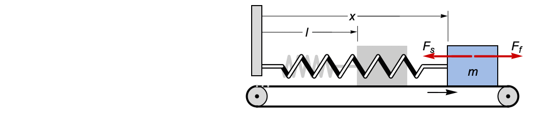
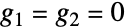
beltv[t_] = vb;
spring[x_] = k(l - x);
friction[v_] := -a(v - beltv[t]);sys := {m x''[t] == spring[x[t]] + friction[x'[t]], x[0] == l, x'[0] == 0};{pos[m_, k_, a_, vb_, t_], vel[m_, k_, a_, vb_, t_]} = DSolveValue[sys, {x[t], x'[t]}, {t, 0, 2}]//FullSimplifyl = 1;
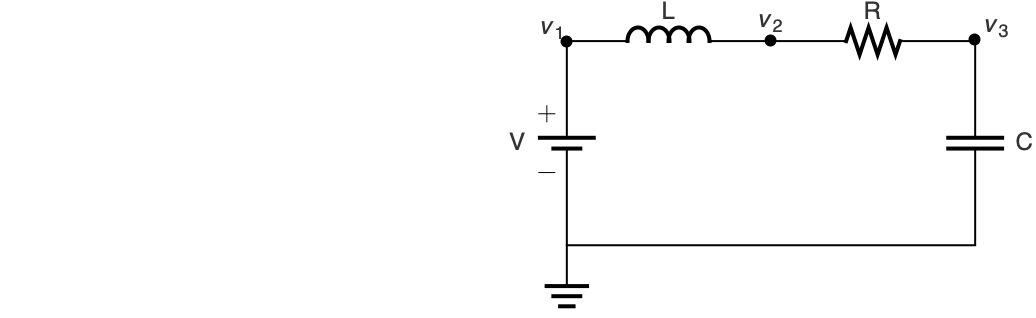
Manipulate[{Plot[{pos[m, k, a, vb, t]}, {t, 0, 2}, PlotRange -> All, PlotLabel -> "Position"], Plot[{vel[m, k, a, vb, t], vb}, {t, 0, 2}, PlotRange -> All, PlotLabel -> "Velocity"]}, {{m, 1, "mass of the block"}, 1, 10, 1}, {{k, 100, "spring constant"}, 100, 1000, 100}, {{vb, 1, "belt velocity"}, 1, 10, 1}, {{a, 5, "friction coefficient"}, 5, 45, 10}, SaveDefinitions -> True]接続に関するキルヒッホフ(Kirchhoff)の法則に加えて構成成分の諸法則を使って,時間

で適用される電圧
のステップインパルスに対するRLC回路の応答のシミュレーションを行う:
ClearAll[r, l, c];
vR[t_] := r iL[t];
vL[t_] := v1[t] - vR[t] - vC[t];
sys = {l iL'[t] == vL[t], c vC'[t] == iL[t]};v1[t_] := UnitStep[t - .01];
ic = {iL[0] == 0, vC[0] == 0};{iL1[r_, c_, l_, t_], vC1[r_, c_, l_, t_]} = DSolveValue[Flatten[{sys, ic}], {iL[t], vC[t]}, t];Manipulate[{Plot[Evaluate[{v1[t], Re[vC1[r, c, l, t]]}], {t, 0, .03}, Filling -> {1 -> 0}, Ticks -> {Range[0.01, 0.03, 0.01], Automatic}, PlotRange -> All, PlotLabel -> "SubscriptBox[V, C][t]"], Plot[Evaluate[Re[iL1[r, c, l, t]]], {t, 0, .03}, Ticks -> {Range[0.01, 0.03, 0.01], Automatic}, PlotRange -> All, PlotLabel -> "I[t]"]}, {{r, 1, "R"}, 1, 10, 1}, {{l, 10^-2, "L"}, 10^-2, 5 10^-2, 10^-2}, {{c, 10^-4, "C"}, 10^-4, 5 10^-4, 10^-4}, SaveDefinitions -> True]水がパイプを通って1つのタンクから別のタンクに流れるときの,2つの円筒形タンクの水位の変化をモデル化する:
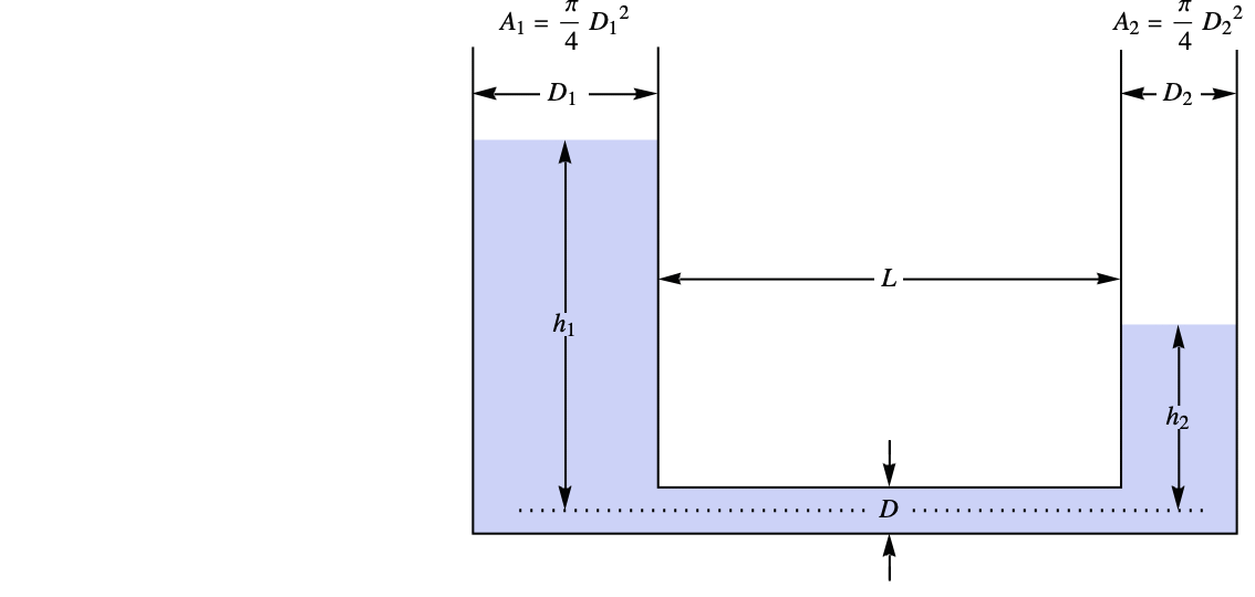
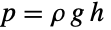
p1[t_] := ρ g h1[t];
p2[t_] := ρ g h2[t];Hagen–Poiseuille関係を使ってパイプの中のフローをモデル化する:
flowRate = (p1[t] - p2[t])(π pipeDia ^ 4) / (128 μ pipeLen);
massConservation = {a1 h1'[t] == -flowRate, a2 h2'[t] == flowRate};
ic = {h1[0] == 1, h2[0] == 0};{h1[t_], h2[t_]} = DSolveValue[Flatten[{massConservation, ic}], {h1[t], h2[t]}, t]params = {pipeLen -> 0.1, pipeDia -> 0.2, a1 -> 1, a2 -> 1, ρ -> 0.2, μ -> 2 10 ^ -3, g -> 9.81};Plot[Evaluate[{h1[t], h2[t]} /. params], {t, 0, 15}, PlotRange -> All, PlotLegends -> {"SubscriptBox[h, 1][t]", "SubscriptBox[h, 2][t]"}]DSolveValue[{CaputoD[x[t], {t, 1.9}] + x[t] == 0, x[0] == 1, x'[0] == 0}, x[t], t]fracsol = Plot[%, {t, 0, 20}]dampedOsc = DSolveValue[{x''[t] + a x'[t] + x[t] == 0, x[0] == 1, x'[0] == 0}, x[t], t]//FullSimplify非整数階振動子のデータを減衰振動子の解にフィットして減衰係数
の対応する値を判定する:
data = Cases[InputForm[fracsol], Line[m_] :> m, -1][[1]];
fit = FindFit[data, dampedOsc, a, t]dampedsol = Plot[dampedOsc /. fit, {t, 0, 20}];
Show[fracsol, dampedsol]LCeqn[α_, l_, c_] = {CaputoD[i[t], {t, α}] + (1/l c)i[t] == 0, i[0] == 0.1, i'[0] == 0};LCsol[α_, l_, c_] := DSolveValue[LCeqn[α, l, c], i[t], t];LCsol[2, l, c]LCsol[1.9, l, c]Plot[Evaluate[{LCsol[2, 1, 1], LCsol[1.9, 1, 1], LCsol[1.8, 1, 1]}], {t, 0, 10}, PlotLegends -> {"α=2", "α=1.9", "α=1.8"}]RCeqn[α_, r_, c_] = {CaputoD[v[t], {t, α}] + (1/r c)v[t] == 0, v[0] == 20};RCsol[α_, r_, c_] := DSolveValue[RCeqn[α, r, c], v[t], t]RCsol[1, r, c]RCsol[0.9, r, c]Plot[Evaluate[{RCsol[1, 10, 1], RCsol[0.9, 10, 1], RCsol[0.8, 10, 1]}], {t, 0, 100}, PlotLegends -> {"α=1", "α=0.9", "α=0.8"}]ハイブリッド微分方程式 (8)
system = {x''[t] + .1x'[t] + x[t] == 0, x[0] == 1, x'[0] == 0};
control = WhenEvent[Mod[t, 1] == 0, x'[t] -> x'[t] + 1];sol = DSolveValue[{system, control}, x, {t, 0, 50}];Plot[Evaluate[{sol[t], sol'[t]}], {t, 0, 50}]sol = DSolveValue[{x''[t] + x[t] == 0, x[0] == 0, x'[0] == 1, WhenEvent[x[t] == 0, x'[t] -> -x'[t]]}, x, {t, 0, 4π}]Plot[Evaluate[{Sin[t], sol[t]}], {t, 0, 4π}]c = .75;
sol = DSolveValue[{y''[t] == -9.8, y[0] == 13.5, y'[0] == 5, a[0] == 13, WhenEvent[y[t] - a[t] == 0, y'[t] -> -c y'[t]], WhenEvent[Mod[t, 1], a[t] -> a[t] - 1]}, {y, a}, {t, 0, 8}, DiscreteVariables -> {a}] ;Plot[Evaluate[{y[t], a[t]} /. Thread[{y, a} -> sol]], {t, 0, 8}, Filling -> {2 -> 0}, Exclusions -> None]正方形の箱の中で,側壁に当るたびに方向を変えるボールをモデル化する:
sol = DSolveValue[{x'[t] == a[t], y'[t] == b[t], x[0] == 0, y[0] == 0, a[0] == 1, b[0] == 17 / 12, WhenEvent[x[t] ^ 2 == 1, a[t] -> -a[t]], WhenEvent[y[t] ^ 2 == 1, b[t] -> -b[t]]}, {x, y}, {t, 0, 50}, DiscreteVariables -> {a, b}];ParametricPlot[{x[t], y[t]} /. Thread[{x, y} -> sol], {t, 0, 50}, Frame -> True, FrameTicks -> None, PlotRange -> 1, Axes -> False]離散時間制御器
で安定化された系
のシミュレーションを行う:
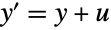
system = {y'[t] == y[t] + u[t], y[0] == 1, u[0] == 0};
control = WhenEvent[Mod[t, 1] == 0, u[t] -> -2y[t]];DSolveValue[{system, control}, {y, u}, {t, 0, 20}, DiscreteVariables -> u];Plot[Evaluate[{u[t], y[t]} /. {Thread[{u, y} -> %]}], {t, 0, 10}, PlotRange -> {-6, 6}, Exclusions -> None]system = {x''[t] == u[t], x[0] == 1, x'[0] == 1, u[0] == -7};τ = 0.5;
control = WhenEvent[Mod[t, τ] == 0, u[t] -> -(1 / τ ^ 2)x[t] - (3 / (2τ))x'[t]];DSolveValue[{system, control}, {x, u}, {t, 0, 2}, DiscreteVariables -> u];Plot[Evaluate[{x[t], x'[t], u[t]} /. Thread[{x, u} -> %]], {t, 0, 2}, PlotRange -> All, Exclusions -> None]system = {x''[t] == u[t], x'[0] == x[0] == 0, u[0] == 1};kp = 1; td = 1;τ = 1; xref = 1;
control = WhenEvent[Mod[t, τ] == 0, u[t] -> kp(xref - x[t] - td x'[t])];DSolveValue[{system, control}, {x, u}, {t, 0, 12}, DiscreteVariables -> u];Plot[Evaluate[{xref, x[t], u[t]} /. Thread[{x, u} -> %]], {t, 0, 12}, Exclusions -> None]sol = DSolveValue[{a'[t] == -1 / 11u[t], a[0] == 1, u[0] == 1,
WhenEvent[a[t] < 0, u[t] -> 0]}, a, {t, 0, 15}, DiscreteVariables -> u]Plot[Evaluate[sol[t]], {t, 0, 15}, PlotRange -> All]遅延微分方程式 (2)
遅延微分方程式によって支配されている動的な系における,カオスの発現を調べる:
sol = DSolveValue[{x'[t] == Sign[x[t - 2]] - x[t - 2], x[t /; t <= 0] == 0.1}, x, {t, 0, 30}];ParametricPlot[Evaluate[{x[t - 2], x[t]} /. {x -> sol}], {t, 2, 30}]f[λ_, μ_] := DSolveValue[{x'[t] == λ x[t] + μ x[t - 1], x[t /; t ≤ 0] == 1 - t}, x[t], {t, 0, 10}]Plot[Evaluate[{f[1 / 2, -1], f[-7 / 2, 4], f[-5, 4]}], {t, 0, 15}, Exclusions -> None]積分方程式 (4)
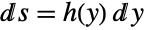
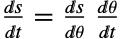
等時曲線問題では,ビーズ玉が,どこに置かれたものであれ,同じ時間で最下点まで落ちる下降曲線を求める必要がある.合計の下降時間を曲線の弧長と速度 v によって表すとアベルの積分方程式
が与えられる.未知の関数
を関係
によって定義し,エネルギー保存の方程式
の変換を使うと明示的な方程式が与えられる:
abeleqn = T == Subsuperscript[∫, 0, y](h[z]/Sqrt[2g]Sqrt[y - z])ⅆz;DSolveValueを使って積分方程式を解く:
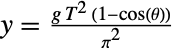
DSolveValue[abeleqn, h[y], y]dxdy = Sqrt[%^2 - 1]積分が実数値であるという仮定のもとに曲線を原点から始めて積分すると,
の関数としての
が与えられる:
x[y_] = Integrate[dxdy, {y, 0, y}, Assumptions -> (2 g T^2 /π^2y) > 1 && y > 0]
と
の値を代入し,ParametricPlotを使って最大等時曲線を表示する:
Show[ParametricPlot[{{x[y], y}, {-x[y], y}} /. {g -> 9.8, T -> 2}, {y, 0, (2(9.8)2^2/π^2)}], ImageSize -> Medium]変数
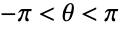
を変更すると,
の範囲での曲線の単純で特異ではないパラメータ化が与えられる:
c[θ_] = (g T^2/π^2){Sin[θ] + θ, 1 - Cos[θ]} ;エネルギーの保存方程式とチェーン規則
を組み合せると,
の関数としての
について次の微分方程式が得られる:
FullSimplify[ (Sqrt[2g (Last[c[θMax]] - Last[c[θ]])] /Sqrt[c'[θ].c'[θ]]) , g > 0 && T > 0]teqn = θ'[t] == (% /. {θ -> θ[t], T -> 2});Θ[t_] = Table[NDSolveValue[{teqn, θ[0] == θMax}, θ[t], {t, 0, 4}], {θMax, {-2 Pi / 3, -Pi / 2, -Pi / 4, -Pi / 12}}];解をプロットするとすべてが2秒で最下点
に達することが分かる:
Plot[Evaluate[Θ[t]], {t, 0, 4}, PlotTheme -> "Scientific"]{cShape[t_], cBeads[t_]} = {c[t], c /@ Θ[t]} /. {T -> 2, g -> 9.8};
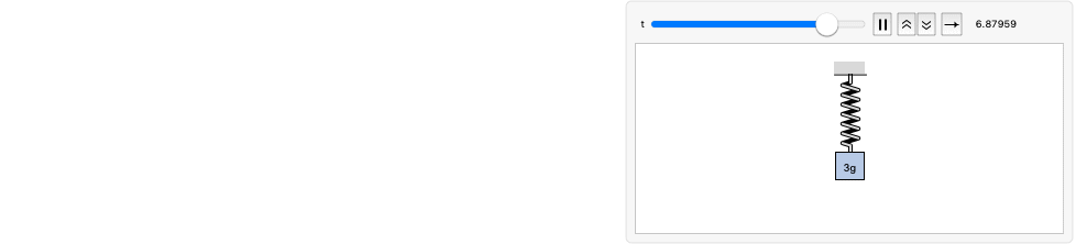
Animate@@{ParametricPlot[cShape[s] , {s, -Pi, Pi}, ImageSize -> Medium, Epilog -> {AbsolutePointSize[8], Point[cBeads[t]]}], {t, 0, 4, Appearance -> "Labeled"}, SaveDefinitions -> True, AnimationDirection -> ForwardBackward}3gの質量が付けられたバネ質量系は3dynes/cmのバネ定数と2g/sの減衰係数を持つ.
で質量が下方に押され,速度28cm/sで下向きに放たれる.
で
の力が質量に対して下向きにかかる.系の速度を時間の関数として求める.速度についての積分方程式は以下で与えられる:
ieqn = 3Derivative[1][v][t] + 2 v[t] + 40 Subsuperscript[∫, 0, t]v[m]ⅆm == 50 Cos[2 t];ic = v[0] == 28;DSolveValueを使って積分微分方程式を解く:
sol = DSolveValue[{ieqn, ic}, v[t], t]Plot[sol, {t, 0, 8}, PlotRange -> All, Filling -> Axis]
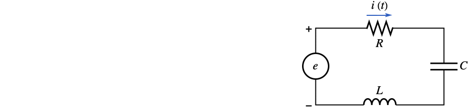
,インダクタンスは,キャパシタンスはである.抵抗器中の電流は最初はである.電流を時間の関数として求める:
ieqn = 5 Derivative[1][i][t] + 0.2 i[t] + (1/0.7)Subsuperscript[∫, 0, t]i[m]ⅆm == 2 Cos[t];ic = i[0] == 1;DSolveValueを使って積分微分方程式を解く:
sol = DSolveValue[{ieqn, ic}, i[t], t]//FullSimplify//ChopPlot[sol, {t, 0, 80}, PlotRange -> All, Filling -> Axis]線形ヴォルテラ積分方程式は線形微分方程式の初期値問題に等しい.この関係を次のヴォルテラ方程式について確かめる:
eqn = y[x] == x^3 + λSubsuperscript[∫, 0, x](t - x)y[t]ⅆt;DSolveValueを使って積分方程式を解く:
sol = DSolveValue[eqn, y[x], x]deqn = D[eqn, {x, 2}]init = {(eqn /. {x -> 0}), (D[eqn, x] /. {x -> 0})}DSolveValue[{deqn, init}, y[x], x]//SimplifyPlot[Table[%, {λ, 1, 3, 0.5}]//Evaluate, {x, 0, 20}, Filling -> Axis]従来の偏微分方程式 (5)
波動方程式を使って,固定長(例えば π)の紐の振動をモデル化する:
eqn = D[u[x, t], {t, 2}] == D[u[x, t], {x, 2}];bc = {u[0, t] == 0, u[π, t] == 0};ic = {u[x, 0] == Sin[m x], Derivative[0, 1][u][x, 0] == 0};dsol = DSolveValue[{eqn, bc, ic}, u[x, t], {x, t}, Assumptions -> Element[m, Integers]]Table[Show[Plot[Table[dsol, {t, 0, 4}]//Evaluate, {x, 0, Pi}, Ticks -> False]], {m, 4}]ic = {u[x, 0] == x(π - x) ^ 2, Derivative[0, 1][u][x, 0] == 0};dsol = DSolveValue[{eqn, bc, ic}, u[x, t], {x, t}] /. {K[1] -> m}Inactive和から4項を抽出する:
sol[x_, t_] = TruncateSum[dsol, 4]Animate[Plot[sol[x, t], {x, 0, π}, PerformanceGoal -> "Quality", PlotRange -> {-5, 5}, ImageSize -> Medium], {t, 0, 12}, SaveDefinitions -> True]2Dで波動方程式を使って半径1の円形皮膜の振動をモデル化する:
eqn = r D[u[r, t], {t, 2}] == D[r D[u[r, t], r], r];bc = u[1, t] == 0;ic = {u[r, 0] == 0, Derivative[0, 1][u][r, 0] == 1};(dsol = DSolveValue[{eqn, bc, ic}, u[r, t], {r, t}])//TraditionalFormInactive和から有限数の項を抽出する:
h[r_, t_] = TruncateSum[dsol, 3]//N;Animate[Plot3D[h[r, t] /. {r -> Sqrt[x ^ 2 + y ^ 2]}, {x, y}∈Disk[], PlotRange -> {-1, 1}, Ticks -> None, Mesh -> True, MeshStyle -> {Red, Blue}, PlotStyle -> Yellow], {t, 0, 4}, SaveDefinitions -> True]熱伝導方程式を使って,長さ1の棒の中の熱の流れをモデル化する:
heqn = D[u[x, t], t] == D[u[x, t], {x, 2}];bc = {u[0, t] == 20, u[1, t] == 50};ic = u[x, 0] == 0;sol = DSolveValue[{heqn, bc, ic}, u[x, t], {x, t}]Inactive和から数項を抽出する:
approxsol = TruncateSum[sol, 3]//ExpandPlot[Table[approxsol, {t, 0.02, 0.5, 0.07}]//Evaluate, {x, 0, 1}, AxesOrigin -> {0, 0}]ssol = DSolveValue[{v''[x] == 0, v[0] == 20, v[1] == 50}, v[x], x]//ExpandPlot[ssol, {x, 0, 1}]heqn = D[u[x, t], t] == D[u[x, t], {x, 2}];bc = {Derivative[1, 0][u][0, t] == 0, Derivative[1, 0][u][1, t] == 0};ic = u[x, 0] == 20 + 80x;sol = DSolveValue[{heqn, bc, ic}, u[x, t], {x, t}]Inactive和から数項を抽出する:
approxsol = TruncateSum[sol, 4]//ExpandPlot[Table[approxsol, {t, 0.02, 0.9, 0.07}]//Evaluate, {x, 0, 1}, AxesOrigin -> {0, 0}, PlotRange -> All]
軸上の実部と虚部の値から始めて複素解析関数を構築する.実部と虚部(u と v)はコーシー・リーマン(Cauchy–Riemann)方程式を満足する:
creqns = {D[u[x, y], x] == D[v[x, y], y], D[v[x, y], x] == -D[u[x, y], y]};xvals = {u[x, 0] == x ^ 3, v[x, 0] == 0};sol[x_, y_] = DSolveValue[{creqns, xvals}, {u[x, y], v[x, y]}, {x, y}]Laplacian[sol[x, y], {x, y}]ContourPlot[sol[x, y], {x, -5, 5}, {y, -5, 5}, ContourStyle -> {Red, Blue}, PlotTheme -> "Marketing"]f[x_, y_] = sol[x, y][[1]] + I sol[x, y][[2]](f[x, y]//Factor) /. {x + I y -> z}一般的な偏微分方程式 (5)
粘度パラメータが無限に小さくなる場合の,極限におけるバーガース方程式の平滑化解の衝撃波への進化を見る:
eqns = { D[u[x, t], t] + u[x, t]D[u[x, t], x] == ϵ D[u[x, t], {x, 2}] , u[x, 0] == Piecewise[{{1, x < 0}}]};dsol = DSolveValue[eqns, u[x, t], {x, t}]Plot3D[dsol /. {ϵ -> 1 / 10}, {x, -2, 2}, {t, 0.001, 5}]Table[Plot3D[dsol /. {ϵ -> 1 / 1000}, {x, -2, 2}, {t, 0.001, 5}, Exclusions -> All, Ticks -> None], {ϵ, {1 / 10, 1 / 100, 1 / 1000}}]//Quiet長さ d の一次元の箱の中で動くように条件付けられた電子は,端点にディリクレ条件がある自由シュレディンガー方程式に支配されている:
eqn = I ℏ D[ψ[x, t], t] == (-ℏ^2/2m) D[ψ[x, t], {x, 2}];
bcs = {ψ[0, t] == 0, ψ[d, t] == 0};DSolveValue[Join[{eqn}, bcs], ψ[x, t], {x, t}]和の中の各項は,正弦を初期状態として使うと確率密度定
が時間依存になるので,常状態と呼ばれる.例えば,以下のようになる:
sol1 = DSolveValue[Join[{eqn, ψ[x, 0] == Sqrt[(2/d)]Sin[Pi(x/d)]}, bcs], ψ[x, t], {x, t}]ρ1[x_, t_] = Simplify[ComplexExpand[Conjugate[sol1]sol1], d > 0]初期データの正規化は,密度の積分(どこかに粒子を発見する全確率)が1になるように選択される:
Integrate[ρ1[x, t], {x, 0, d}]上記以外の初期条件を使うと,たとえ2つの定常状態の和のように単純なものでも,結果として複雑な時間依存密度になる:
sol2 = DSolveValue[Join[{eqn, ψ[x, 0] == (1/Sqrt[d])Sin[Pi(x/d)] + (1/Sqrt[d])Sin[2Pi(x/d)]}, bcs], ψ[x, t], {x, t}]ρ2[x_, t_] = Simplify[ComplexExpand[Conjugate[sol2]sol2], d > 0]Integrate[ρ2[x, t], {x, 0, d}]電子質量と
の値をSI単位で入れ,d をよく使われる原子間距離の1nmに設定すると,次の密度関数になる:
ρe[x_, t_] = ρ2[x, t] /. {ℏ -> 1.055*^-34, m -> 9.109 * 10 ^ -31, d -> 10 ^ -9}Plot3D[ρe[x 10^-9, t 10^-15]10^-9, {x, 0, 1}, {t, 0, 3.66}, PlotTheme -> {"Grid", "LargeLabels"}, AxesLabel -> {"x (nm)", "t (fs)", "ρe (SuperscriptBox[nm, -1])"}, ImageSize -> Medium]このグラフを確率密度の動画として見ると,電子の「中心」がボックスの片側からもう片側に動くのが分かる:
Animate[Plot[ρe[x, t], {x, 0, 10 ^ -9}, PerformanceGoal -> -"Quality", PlotRange -> {0, 4*^9}, ImageSize -> Medium, AxesLabel -> {"x (m)", "ρe (SuperscriptBox[m, -1])"}], {t, 0, 3.66*^-15}, SaveDefinitions -> True]ブラック・ショールズモデルを使って,もとになっている資産価格と行使価格の両方が100ドル,安全金利5%,もとになっている資産のボラティリティが20%,満期1年の場合の,ヨーロッパバニラコールオプションの値を求める:
BlackScholesModel = {D[c[t, s], t] + 1 / 2σ ^ 2 s ^ 2 D[c[t, s], {s, 2}] + r s D[c[t, s], s] - r c[t, s] == 0, c[T, s] == Max[s - k, 0]};dsol = DSolveValue[BlackScholesModel, c[t, s], {t, s}]dsol /. {t -> 0, s -> 100, k -> 100, σ -> 0.2, T -> 1, r -> 0.05}FinancialDerivativeで与えられた値と比較する:
FinancialDerivative[{"European", "Call"}, {"StrikePrice" -> 100.00, "Expiration" -> 1}, {"InterestRate" -> 0.05, "Volatility" -> 0.2, "CurrentPrice" -> 100}]sol = DSolveValue[{D[f[x, y], x] == x y Cos[x y] + Sin[x y],
D[f[x, y], y] == -E^-y + x^2 Cos[x y]}, f[x, y], {x, y}]Plot3D[Table[sol /. {C[1] -> k}, {k, 1, 22, 5}]//Evaluate, {x, 0, 10}, {y, 0, 2}, PlotRange -> All]コーシー問題を解き,スターリング(Stirling)数を生成する:
sol = DSolveValue[{(1 - x)D[u[x, y], x] == y u[x, y], u[0, y] == 1}, u[x, y], {x, y}]Table[(-1) ^ i SeriesCoefficient[ Series[sol, {x, 0, 10}, {y, 0, 4}], {10, i}]10!, {i, 4}]StirlingS1[10, Range[4]]系のモデル (5)
tfm = TransferFunctionModel[{{{1}}, 5 + s + s^2}, s];ir[τ_] = DSolveValue[tfm, "ImpulseResponse", τ]UnilateralConvolveを使って正弦波入力からのモデルの出力応答を得る:
lconv[t_] = UnilateralConvolve[ir[τ], Sin[τ], τ, t]次は,インパルス応答と正弦波関数のラプラスたたみ込みを示している:
Animate[
GraphicsRow[{
Plot[{ir[τ], Sin[t - τ]}, {τ, 0, 2Pi}, ...],
Plot[ir[τ] Sin[t - τ]UnitStep[t - τ], {τ, 0, 2Pi}, ...],
Plot[lconv[τ], {τ, 0, t}, ...]}, ImageSize -> 480], {t, 0, 2Pi}]正弦波入力からの出力応答をDSolveValueを使って計算する:
or = DSolveValue[{Sin[t] -> tfm}, "OutputResponse", t]or - lconv[t]//FullSimplify単位ステップ入力に応じて,安定した1次系の定常状態の出力値を決定する:
y = DSolveValue[TransferFunctionModel[{{{1}}, 1 + 10*s}, s], "StepResponse", t];Subscript[y, ss] = Limit[y, t -> ∞]τ = t /. FindRoot[y == (1 - (1/E)) Subscript[y, ss], {t, 1}]With[{y1 = y /. t -> τ}, Plot[y, {t, 0, 40}, Epilog -> {Dashed, Line[{{τ, 0}, {τ, y1}, {0, y1}}], PointSize[Medium], Point[{{τ, y1}}]}]]ssm = StateSpaceModel[{{{0, 0, -10, 0}, {0, 0, 0, 10}, {3.7, 0, -2, 0}, {0, -0.6, 0, -5}},
{{0, 0}, {0, 0}, {8.533, 0}, {0, 8.533}}, {{0.5, 0.5, 0, 0}, {-2.113, 2.113, 0.375, 0.375}},
{{0, 0}, {0, 0}}}, SamplingPeriod -> None, SystemsModelLabels -> None];MapIndexed[Plot[#, {t, 0, 5}, PlotRange -> All, PlotLabel -> "Input " <> ToString@First@#2 <> " -> " <> " State " <> ToString@Last@#2]&, DSolveValue[UnitStep[t] -> ssm, "StateResponse", t]//Simplify//Chop, {2}]望ましい生産率と販売率を入力として,実際の生産率と在庫レベルを状態として持つ生産および在庫システムモデルの状態空間モデル:
ssm = StateSpaceModel[{{{-1, -0.1875}, {1, 0}}, {{0.1875, 0}, {0, -1}}}, SamplingPeriod -> None,
SystemsModelLabels -> None];特定の生産率と初期の平衡状態からの売上の10%の増加に対する応答を決定する:
resp = DSolveValue[{{Subscript[u, 1], 1.1 Subscript[x, 10]} -> ssm, {Subscript[x, 10], Subscript[u, 1]}}, "StateResponse", t]//Expand//ChopPlot[Evaluate[resp] /. {Subscript[x, 10] -> 1, Subscript[u, 1] -> 6}, {t, 0, 50}, PlotStyle -> {Thickness[0.005], Dashing[{0.05, 0.01}]}, PlotRange -> All, AxesOrigin -> {0, 0}, PlotLabel -> "State response", AxesLabel -> {"t"}]Clohessy–Wiltshire方程式は,中心体を周回する2つの衛星間の相対運動をモデル化する:
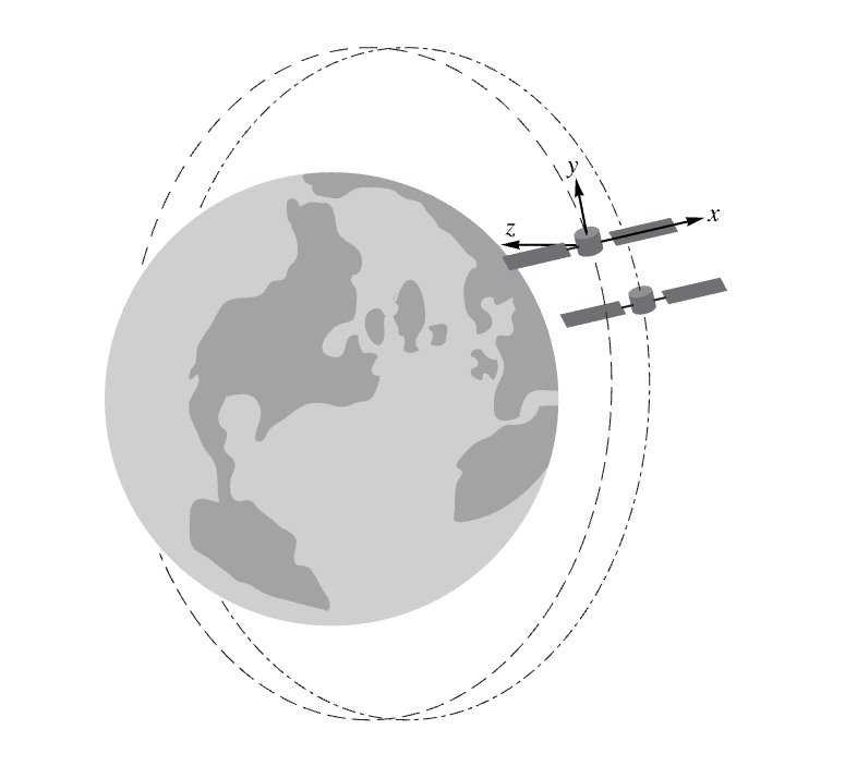
sat = StateSpaceModel[{{{0, 1, 0, 0, 0, 0}, {3*n^2, 0, 0, 2*n, 0, 0},
{0, 0, 0, 1, 0, 0}, {0, -2*n, 0, 0, 0, 0}, {0, 0, 0, 0, 0, 1},
{0, 0, 0, 0, -n^2, 0}}, {{0, 0, 0}, {1, 0, 0}, {0, 0, 0}, {0, 1, 0}, {0, 0, 0},
{0, 0, 1}}, {{1, 0, 0, 0, 0, 0}, {0, 1, 0, 0, 0, 0}, {0, 0, 1, 0, 0, 0}},
{{0, 0, 0}, {0, 0, 0}, {0, 0, 0}}}, SamplingPeriod -> None, SystemsModelLabels -> None];DSolveValueを使って,打上げ条件の特定の集合から閉じた相対軌道を得る:
n = 0.001;Subscript[x, 0] = 1;Subscript[xd, 0] = 0.0005;
x = Map[DSolveValue[{{0, 0, 0} -> sat, {Subscript[x, 0], Subscript[xd, 0], (2Subscript[xd, 0]/n), -2n Subscript[x, 0], Sequence@@##}}, "StateResponse", {t, 0, 5 (2Pi/n)}]&, {{-2 Subscript[x, 0], -2 Subscript[xd, 0]}, {2 Subscript[x, 0], 2 Subscript[xd, 0]}}];ParametricPlot3D[{x[[1, 1 ;; 5 ;; 2]], x[[2, 1 ;; 5 ;; 2]]}, {t, 0, 5 (2Pi/n)}, BoxRatios -> {1, 1, 1}, AxesLabel -> {"X", "Y", "Z"}]特性と関係 (12)
DSolveValueは解の式を返す:
DSolveValue[{y'[x] == y[x], y[0] == 1}, y[x], x]DSolveは解についての規則を返す:
DSolve[{y'[x] == y[x], y[0] == 1}, y[x], x]sol = DSolveValue[{y''[x] - y[x] == 0, y[0] == 1, y'[0] == 4}, y, x]Simplify[{y''[x] - y[x] == 0, y[0] == 1, y'[0] == 4} /. y -> sol]Integrateに対応する微分方程式:
DSolveValue[y'[x] == Exp[x ^ 2], y[x], x]Integrate[Exp[x ^ 2], x]NDSolveValueを使って数値解を求める:
exactsol = DSolveValue[{y''[x] + y[x] == 0, y[0] == 1, y'[0] == 0}, y, x]Table[exactsol[x], {x, -2., 2}]numsol = NDSolveValue[{y''[x] + y[x] == 0, y[0] == 1, y'[0] == 0}, y, {x, -2, 2}]Table[numsol[x], {x, -2., 2}]AsymptoticDSolveValueを使って漸近展開を求める:
dsol = DSolveValue[{y'[x] - 2y[x] == 0, y[0] == 1}, y[x], x]Series[%, {x, 0, 4}]//NormalAsymptoticDSolveValue[{y'[x] - 2y[x] == 0, y[0] == 1}, y[x], {x, 0, 4}]DEigensystemを使って固有値と固有関数を求める:
{ℒ, ℬ} = {-Laplacian[u[x], {x}], DirichletCondition[u[x] == 0, True]};DSolveValue[{u''[x] + λ u[x] == 0, u[0] == 0, u[π] == 0}, u[x], x]DEigensystem[{ℒ, ℬ}, u[x], {x, 0, Pi}, 3]DSolveValueを使ってインパルス応答を計算する:
DSolveValue[y'''[x] - 5y''[x] + 9y'[x] - 5y[x] == DiracDelta''[x] + 2DiracDelta'[x] + DiracDelta[x] && y[-1] == 0 && y'[-1] == 0 && y''[-1] == 0, y[x], x]//FullSimplifyInverseLaplaceTransformを使った同じ計算:
InverseLaplaceTransform[(s ^ 2 + 2s + 1/s ^ 3 - 5s ^ 2 + 9s - 5), s, x]//FullSimplify記号解が得られなかったときには,N[DSolveValue[…]]を適用してNDSolveValueを呼び出す:
DSolveValue[{y''[x] + x ^ 2 y'[x] + Tan[y[x]] == 1, y[0] == 1, y'[0] == 1}, y, {x, 0, 1}]sol = N[%]Table[sol[x], {x, 0, 1, 0.2}]CompleteIntegralは非線形偏微分方程式の完全積分を求める:
deqn = D[u[x, y], x] + D[u[x, y], y] ^ 2 == 3;CompleteIntegral[deqn, u[x, y], {x, y}]DSolveValueは同じ解を警告メッセージとともに返す:
DSolveValue[deqn, u[x, y], {x, y}]CompleteIntegralを使って線形偏微分方程式の完全積分を求める:
deqn = D[u[x, y], x] + 2D[u[x, y], y] == 1;CompleteIntegral[deqn, u[x, y], {x, y}]DSolveValueはこの偏微分方程式についての一般解を返す:
DSolveValue[deqn, u[x, y], {x, y}]DFixedPointsを使って2つの常微分方程式系の固定点を求める:
DFixedPoints[{x'[t] == -x[t] - y[t] - 1, y'[t] == 2x[t] - y[t] + 5}, {x, y}, t]DStabilityConditionsを使って固定点の安定性を解析する:
DStabilityConditions[{x'[t] == -x[t] - y[t] - 1, y'[t] == 2x[t] - y[t] + 5}, {x, y}, t]DSolveValue[{x'[t] == -x[t] - y[t] - 1, y'[t] == 2x[t] - y[t] + 5, x[0] == -2, y[0] == 1}, {x[t], y[t]}, t]//Simplifysol = DSolveValue[{x'[t] == -x[t] - y[t] - 1, y'[t] == 2x[t] - y[t] + 5, x[0] == 3, y[0] == -2}, {x[t], y[t]}, t]//SimplifyPlot[Evaluate[sol], {t, 0, 20}]sim = SystemModelSimulate[[image]]SystemModelPlot[sim]考えられる問題 (5)
DSolveValueは,解に複数の分岐がある場合は,単一の分岐だけを返す:

DSolveValue[{y'[x] + y[x] == Sin[x], y'[0] ^ 2 == 1}, y[x], x]DSolveを使って解のすべての分岐を得る:
DSolve[{y'[x] + y[x] == Sin[x], y'[0] ^ 2 == 1}, y[x], x]sol = DSolveValue[y'[x] == f[x], y[x], x]sol /. f -> Function[x, 0]Activateを使って積分を評価する:
Activate[%]DSolveValue[x'[K] == K ^ K, x[K], K]DSolveValue[x'[C] == C ^ C, x[C], C]DSolveValue[x'[k] == k ^ k, x[k], k]DSolveValue[x'[c] == c ^ c, x[c], c]y[x_] := Cos[x]DSolveValue[{y'[x] == 0, y[0] == 1}, y, x]Clear[y]DSolveValue[{y'[x] == 0, y[0] == 1}, y[x], x]eqn = y''[x] + (k + g1 / (a + x)) y'[x] + (m + g2 / (a + x)) y[x] == 0;sol = DSolveValue[eqn, y[x], x]得られた解はパラメータの特定の値
についての常微分方程式の一般解ではない:
sol /. {g1 -> 0, g2 -> 0}//Simplifyこの場合の一般解は,まず方程式に代入することで得ることができる:
DSolveValue[eqn /. {g1 -> 0, g2 -> 0}, y[x], x]おもしろい例題 (2)
{x, y, t} = DSolveValue[{x'[s] == Cos[t[s]], y'[s] == Sin[t[s]], t'[s] == s, x[0] == 0, y[0] == 0, t[0] == 0}, {x, y, t}, s]ParametricPlot[{x[s], y[s]}, {s, -10, 10}]ルジャンドル(Legendre)微分演算子の六次対称ベキを解く:
sol = DSolveValue[(-((192n(1 + n)x ^ 5) / (1 - x ^ 2) ^ 6) + (2496n(1 + n)x ^ 3) / (1 - x ^ 2) ^ 5 - (8160n ^ 2(1 + n) ^ 2x ^ 3) / (1 - x ^ 2) ^ 5 - (1632n(1 + n)x) / (1 - x ^ 2) ^ 4 + (7824n ^ 2(1 + n) ^ 2x) / (1 - x ^ 2) ^ 4 - (6912n ^ 3(1 + n) ^ 3x) / (1 - x ^ 2) ^ 4)y[x] + ((64x ^ 6) / (1 - x ^ 2) ^ 6 - (1824x ^ 4) / (1 - x ^ 2) ^ 5 + (8256n(1 + n)x ^ 4) / (1 - x ^ 2) ^ 5 + (2880x ^ 2) / (1 - x ^ 2) ^ 4 - (19200n(1 + n)x ^ 2) / (1 - x ^ 2) ^ 4 + (22896n ^ 2(1 + n) ^ 2x ^ 2) / (1 - x ^ 2) ^ 4 - 272 / (1 - x ^ 2) ^ 3 + (2208n(1 + n)) / (1 - x ^ 2) ^ 3 - (4384n ^ 2(1 + n) ^ 2) / (1 - x ^ 2) ^ 3 + (2304n ^ 3(1 + n) ^ 3) / (1 - x ^ 2) ^ 3)
y'[x] + (-((2016x ^ 5) / (1 - x ^ 2) ^ 5) + (9408x ^ 3) / (1 - x ^ 2) ^ 4 - (19488n(1 + n)x ^ 3) / (1 - x ^ 2) ^ 4 - (3696x) / (1 - x ^ 2) ^ 3 + (12768n(1 + n)x) / (1 - x ^ 2) ^ 3 - (9408n ^ 2(1 + n) ^ 2x) / (1 - x ^ 2) ^ 3)y''[x] + ((4816x ^ 4) / (1 - x ^ 2) ^ 4 - (7168x ^ 2) / (1 - x ^ 2) ^ 3 + (9632n(1 + n)x ^ 2) / (1 - x ^ 2) ^ 3 + 616 / (1 - x ^ 2) ^ 2 - (1456n(1 + n)) / (1 - x ^ 2) ^ 2 + (784n ^ 2(1 + n) ^ 2) / (1 - x ^ 2) ^ 2)y'''[x] + (-((2800x ^ 3) / (1 - x ^ 2) ^ 3) + (1400x) / (1 - x ^ 2) ^ 2 - (1400n(1 + n)x) / (1 - x ^ 2) ^ 2)
y''''[x] + ((560x ^ 2) / (1 - x ^ 2) ^ 2 - 70 / (1 - x ^ 2) + (56n(1 + n)) / (1 - x ^ 2))y'''''[x] - (42x y''''''[x]) / (1 - x ^ 2) + y'''''''[x] == 0, y[x], x]テクニカルノート
履歴
2014 で導入 (10.0) | 2015 で更新 (10.3) ▪ 2016 (11.0) ▪ 2017 (11.2) ▪ 2019 (12.0) ▪ 2021 (13.0) ▪ 2022 (13.2) ▪ 2024 (14.0) ▪ 2025 (14.2) ▪ 2026 (15.0)
テキスト
Wolfram Research (2014), DSolveValue, Wolfram言語関数, https://reference.wolfram.com/language/ref/DSolveValue.html (2026年に更新).
CMS
Wolfram Language. 2014. "DSolveValue." Wolfram Language & System Documentation Center. Wolfram Research. Last Modified 2026. https://reference.wolfram.com/language/ref/DSolveValue.html.
APA
Wolfram Language. (2014). DSolveValue. Wolfram Language & System Documentation Center. Retrieved from https://reference.wolfram.com/language/ref/DSolveValue.html
BibTeX
@misc{reference.wolfram_2026_dsolvevalue, author="Wolfram Research", title="{DSolveValue}", year="2026", howpublished="\url{https://reference.wolfram.com/language/ref/DSolveValue.html}", note=[Accessed: 09-September-2026]}
BibLaTeX
@online{reference.wolfram_2026_dsolvevalue, organization={Wolfram Research}, title={DSolveValue}, year={2026}, url={https://reference.wolfram.com/language/ref/DSolveValue.html}, note=[Accessed: 09-September-2026]}