AbsArgPlot[f,{x,xmin,xmax}]
AbsArgPlot[{f1,f2,…},{x,xmin,xmax}]
複数の関数をプロットする.
AbsArgPlot[{…,w[fi],…},…]
記号ラッパー w で定義された特徴で fiをプロットする.
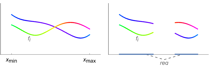
AbsArgPlot[…,{x}∈reg]
変数 x が幾何領域 reg にあるとみなす.
AbsArgPlot
AbsArgPlot[f,{x,xmin,xmax}]
AbsArgPlot[{f1,f2,…},{x,xmin,xmax}]
複数の関数をプロットする.
AbsArgPlot[{…,w[fi],…},…]
記号ラッパー w で定義された特徴で fiをプロットする.
AbsArgPlot[…,{x}∈reg]
変数 x が幾何領域 reg にあるとみなす.
詳細とオプション
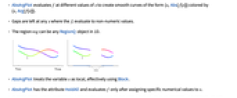
- AbsArgPlotは x のさまざまな値で f を評価して,{x,Arg[f[x]]}で彩色された{x,Abs[f[x]]}という形の滑らかな曲線を作る.
- fiを評価しても数値にならなかった任意の x については空白が残される.
- 領域 reg は1Dの任意のRegionQオブジェクトでよい.
- AbsArgPlotは,事実上Blockを使って,変数 x を局所的なものとして扱う.
- AbsArgPlotには属性HoldAllがあり,x に特定の数値を割り当てた後ではじめて f を評価する.
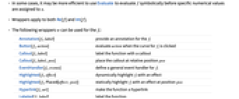
- 場合によっては,x に特定の数値が割り当てられる前に,Evaluateを使って f を記号的に評価した方がより効率的かもしれない.
- ラッパーは,Re[f]とIm[f]の両方に適用される.
- fiには次のラッパー w を使うことができる.
-
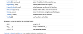
Annotation[fi,label] fiの注釈を与える Button[fi,action] fiの曲線がクリックされたときに action を評価する Callout[fi,label] コールアウトで関数にラベルを付ける Callout[fi,label,pos] 相対的な位置 pos にコールアウトを置く EventHandler[fi,events] fiについての一般的なイベントハンドラを定義する Highlighted[fi,effect] 効果を使って fiを動的にハイライトする Highlighted[fi,Placed[effect,pos]] 位置 pos で効果を使って fiを静的にハイライトする Hyperlink[fi,uri] 関数をハイパーリンクにする Labeled[fi,label] 関数にラベルを付ける Labeled[fi,label,pos] 相対的な位置 pos にラベルを置く Legended[fi,label] 凡例で関数を識別する PopupWindow[fi,cont] 関数にポップアップウィンドウを付ける StatusArea[fi,label] マウスオーバーの際にステータスエリアに表示する Style[fi,styles] 関数を指定されたスタイルで表示する Tooltip[fi,label] 関数にツールチップを付ける Tooltip[fi] 関数をツールチップとして使う - ラッパー w は複数のレベルに適用することができる.
-
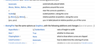
w[fi] fiをラップする w[{f1,…}] fiの集合をラップする w1[w2[…]] ネストしたラッパーを使う - Callout,Labeled,Placedには次の位置 pos を使うことができる.
-
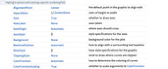
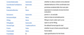
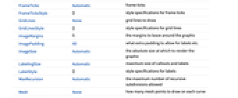
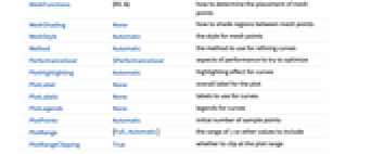
Automatic 自動的に置かれたラベル Above, Below, Before, After 曲線の周囲の位置 x 位置 x における曲線の近く Scaled[s] 曲線に沿ったスケールされた位置 s {s,Above},{s,Below},… 曲線に沿った位置 s における相対的な位置 {pos,epos} 曲線の相対的な位置 pos に置かれたラベル中の epos - AbsArgPlotにはGraphicsと同じオプションに以下の追加・変更を加えたものが使える. [全オプションのリスト]
- 次は,ClippingStyleの可能な設定である.
-

Automatic 切り取られた部分に破線を使う 

None 曲線の切り取られた部分は省略する 

style 切り取られた部分に style を使う - デフォルト設定のExclusions->AutomaticとExclusionsStyle->Noneでは,AbsArgPlotはそれが検出した不連続な箇所および特異点で曲線を分割する.Exclusions->Noneとすると不連続な箇所や特異点でも曲線は繋がれる.
- Exclusions->{x1,x2,…}はExclusions->{x==x1,x==x2,…}に等しい.
- PlotLabels->"Expressions"はラベルのテキストとして fiを使う.
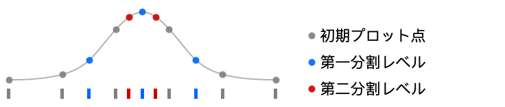
- AbsArgPlotは,まず,PlotPointsで指定された,等間隔の数多くのサンプル点で f を評価する.次に,適応的アルゴリズムを使って,最大でMaxRecursion回,指定された区間をさらに分割して,追加的なサンプル点を選ぶ.
- 有限数のサンプル点しか使われないので,AbsArgPlotが f の特徴を見逃すことも起こり得る.PlotPointsとMaxRecursionの設定値を大きくすると,そのような特徴が検出できることが多い.
- 次は,曲線に影響するテーマである.
-

"ThinLines" 細いプロット線 

"MediumLines" 中太のプロット線 

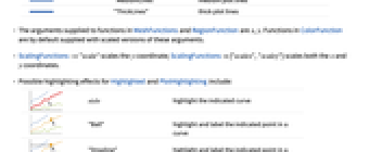
"ThickLines" 太いプロット線 - MeshFunctionsとRegionFunctionの関数に与えられる偏角は,x と y である.ColorFunctionの関数には,デフォルトで,これらの偏角のスケールされたバージョンが与えられる.
- ScalingFunctions->"scale"は
座標をスケールし,ScalingFunctions{"scalex","scaley"}は
座標と
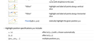
座標の両方をスケールする. - HighlightedとPlotHighlightingの可能な効果には以下がある.
-
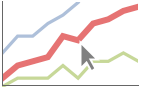
style 指定の曲線をハイライトする 

"Ball" 曲線上の指定の点をハイライトしてラベルを付ける 
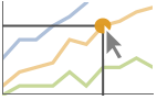
"Dropline" 曲線上の指定の点を軸までのドロップラインでハイライトしてラベルを付ける 

"XSlice" 垂直スライスに沿ったすべての点をハイライトしてラベルを付ける 
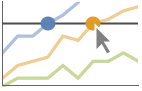
"YSlice" 水平スライスに沿ったすべての点をハイライトしてラベルを付ける 

Placed[effect,pos] 指定の点 pos を静的にハイライトする - 位置指定 pos のハイライトには以下がある.
-
x, {x} {x,y}における効果,y は自動的に選択される {x,y} {x,y}における効果 {pos1,pos2,…} 複数の位置 posi
全オプションのリスト
例題
すべて開く すべて閉じる例 (6)
偏角によって彩色された,実変数の複素関数の絶対値をプロットする:
AbsArgPlot[Sin[I x] + Sin[Pi x], {x, -2, 2}]AbsArgPlot[{Sin[I x] + Sin[Pi x], 2Exp[I π x]}, {x, -2, 2}]AbsArgPlot[{Sin[I x] + Sin[Pi x], 2Exp[I π x]}, {x, -2, 2}, PlotLabels -> "Expressions"]AbsArgPlot[{Sin[I x] + Sin[Pi x], 2Exp[I π x]}, {x, -2, 2}, PlotLegends -> Automatic]AbsArgPlot[Sin[I x] + Sin[Pi x], {x, -2, 2}, Filling -> Axis]PlotとAbsArgPlotを比較する:
{
{Plot[Abs[Sin[x] + Sin[I Sin[3x]]], {x, -Pi, Pi}], Plot[Arg[Sin[x] + Sin[I Sin[3x]]], {x, -Pi, Pi}, ColorFunction -> Hue]},
AbsArgPlot[Sin[x] + Sin[I Sin[3x]], {x, -Pi, Pi}]}スコープ (18)
サンプリング (8)
関数の変化が大きいところでは,より多くの点のサンプルが取られる:
AbsArgPlot[Sin[x] + Sin[I Sin[3x]], {x, 0, 4Pi}]AbsArgPlot[1 + Exp[-Abs[x]]Sin[I Sin[5x]], {x, -Pi, Pi}]AbsArgPlot[I + Floor[Sqrt[x]], {x, -100, 100}]Exclusions->Noneを使って曲線を繋げる:
AbsArgPlot[I + Floor[Sqrt[x]], {x, -100, 100}, Exclusions -> None]PlotPointsとMaxRecursionを使って適応的サンプリングを制御する:
Grid@Table[AbsArgPlot[Sin[I x] + Sin[Pi x], {x, -2, 2}, PlotPoints -> pp, MaxRecursion -> mr], {mr, {0, 1, 2}}, {pp, {15, 30}}]𝒟 = ImplicitRegion[-2 ≤ x ≤ 1 / 2∨1 ≤ x ≤ 2, {x}];AbsArgPlot[Sin[I x] + Sin[Pi x], {x}∈𝒟]MeshRegionを使って定義域を指定する:
𝒟 = MeshRegion[{{-2}, {-1}, {-1 / 2}, {1 / 2}, {1}, {2}}, Line[{{1, 2}, {3, 4}, {5, 6}}]];AbsArgPlot[Sin[x^2] - I, {x}∈𝒟]AbsArgPlot[{Sin[x] / x, 1 / x, -1 / x}, {x, -Infinity, Infinity}]ラベルと凡例 (5)
AbsArgPlot[{ArcCos[x], ArcSin[x]}, {x, -3, 3}, PlotLegends -> Automatic]AbsArgPlot[{ArcCos[x], ArcSin[x]}, {x, -3, 3}, PlotLabels -> Automatic]AbsArgPlot[{Callout[ArcCos[x]], Tooltip[ArcSin[x]]}, {x, -3, 3}]曲線には,通常,マウスオーバーの際の座標を示すインタラクティブなコールアウトが付いている:
AbsArgPlot[x^2 - 4, {x, -5, 5}]{AbsArgPlot[{x^2 - 4, Sinc[x]}, {x, -3, 3}, PlotHighlighting -> "Dropline"], AbsArgPlot[{x^2 - 4, Sinc[x]}, {x, -3, 3}, PlotHighlighting -> "XSlice"]}プレゼンテーション (5)
AbsArgPlot[{ArcSin[x], ArcCos[x]}, {x, -3, 3}, PlotStyle -> {Thick, Dashed}]AbsArgPlot[{ArcSin[x], ArcCos[x]}, {x, -3, 3}, AxesLabel -> {x, ""}, PlotLabels -> Automatic, PlotLegends -> Automatic]AbsArgPlot[Sin[x] + Sin[I Sin[3x]], {x, -Pi, Pi}, Filling -> {1 -> Axis}]AbsArgPlot[{ArcSin[x], 3Exp[I x] + 0.5Exp[5I x]}, {x, -3, 3}, PlotTheme -> "Business"]ScalingFunctionsを使って軸をスケールする:
AbsArgPlot[x + I Exp[x], {x, -5, 5}, ScalingFunctions -> "Log"]オプション (113)
AspectRatio (4)
デフォルトで,AbsArgPlotはプロットに固定した縦横比を使用する:
AbsArgPlot[x^2 - 4, {x, -4, 4}]AspectRatio1として縦と横の長さを等しくする:
AbsArgPlot[x^2 - 4, {x, -4, 4}, AspectRatio -> 1]AspectRatioAutomaticはプロット範囲から比率を決定する:
AbsArgPlot[x^2 - 4, {x, -4, 4}, AspectRatio -> Automatic]AspectRatioFullは他の構造物の中にぴったり収まるように縦横比を調整する:
plot = AbsArgPlot[x^2 - 4, {x, -4, 4}, AspectRatio -> Full];{Framed[Pane[plot, {50, 100}]], Framed[Pane[plot, {100, 100}]], Framed[Pane[plot, {100, 50}]]}Axes (4)
デフォルトで.AbsArgPlotにはAxesが描かれる:
AbsArgPlot[x^2 - 4, {x, -4, 4}]軸の代りにFrameを使う:
AbsArgPlot[x^2 - 4, {x, -4, 4}, Axes -> False, Frame -> True]AxesOriginを使って軸の交点を指定する:
AbsArgPlot[x^2 - 4, {x, -4, 4}, AxesOrigin -> {0, 0}]{AbsArgPlot[x^2 - 4, {x, -4, 4}, Axes -> {True, False}], AbsArgPlot[x^2 - 4, {x, -4, 4}, Axes -> {False, True}]}AxesLabel (3)
AxesOrigin (2)
AxesStyle (4)
AbsArgPlot[x^2 - 4, {x, -4, 4}, AxesStyle -> Red]AbsArgPlot[x^2 - 4, {x, -4, 4}, AxesStyle -> {Directive[Thick, Brown], Directive[Thick, Blue]}]AbsArgPlot[x^2 - 4, {x, -4, 4}, AxesStyle -> Blue, TicksStyle -> Red]AbsArgPlot[x^2 - 4, {x, -4, 4}, AxesStyle -> Blue, LabelStyle -> Red]ClippingStyle (2)
ColorFunction (4)
AbsArgPlot[Sin[I x] + Sin[Pi x], {x, -2, 2}]AbsArgPlot[Sin[I x] + Sin[Pi x], {x, -2, 2}, ColorFunction -> "AvocadoColors"]ColorFunctionはPlotStyleよりも優先順位が高い:
AbsArgPlot[Sin[I x] + Sin[Pi x], {x, -2, 2}, ColorFunction -> "AvocadoColors", PlotStyle -> Directive[Red, Dashed]]AbsArgPlot[Sin[I x] + Sin[Pi x], {x, -2, 2}, ColorFunction -> Function[{arg}, If[arg ≤ 0, Red, Green]], PlotStyle -> Thick, ColorFunctionScaling -> False]ColorFunctionScaling (1)
Exclusions (3)
ExclusionStyle (1)
Filling (4)
Table[AbsArgPlot[Sin[I x] + Sin[Pi x], {x, -3, 3}, Filling -> f], {f, {Axis, Top, Bottom, 3}}]複数の曲線が指定されている場合は,塗潰しに透明な色が使われる:
AbsArgPlot[{Sin[I x] + Sin[Pi x], 2Exp[I π x]}, {x, -2, 2}, Filling -> Axis]AbsArgPlot[{ArcSin[x], 3Exp[I x] + 0.5Exp[5I x]}, {x, -3, 3}, Filling -> {1 -> Axis}]AbsArgPlot[{Sin[I x] + Sin[Pi x], 2Exp[I π x]}, {x, -2, 2}, Filling -> {1 -> {2}}]FillingStyle (2)
Table[AbsArgPlot[{ArcSin[x], 3Exp[I x] + 0.5Exp[5I x]}, {x, -3, 3}, Filling -> {1 -> Axis}, FillingStyle -> c], {c, {Red, Green, Blue, Yellow}}]2本の曲線の間を,2番目の曲線の下を赤で,上を青で塗り潰す:
AbsArgPlot[{ArcSin[x], Exp[I x] + 0.5Exp[5I x]}, {x, -3, 3}, Filling -> {1 -> {2}}, FillingStyle -> {Red, Blue}]Frame (3)
AbsArgPlot[x Sin[1 / x], {x, -.25, .25}, Frame -> True]AbsArgPlot[x Sin[1 / x], {x, -.25, .25}, Frame -> {{True, True}, {False, False}}]AbsArgPlot[x Sin[1 / x], {x, -.25, .25}, Frame -> {{False, False}, {True, True}}]FrameLabel (2)
FrameStyle (2)
AbsArgPlot[x Sin[1 / x], {x, -.25, .25}, Frame -> True, FrameStyle -> Directive[StandardBlue, Thick]]AbsArgPlot[x Sin[1 / x], {x, -.25, .25}, Frame -> True, FrameStyle -> {{Directive[Green, Thick], Directive[Red]}, {Directive[Gray, Thick], Directive[Blue]}}]FrameTicks (8)
デフォルトで,FrameTicksは自動的に置かれる:
AbsArgPlot[x Sin[1 / x], {x, -.25, .25}, Frame -> True]AbsArgPlot[x Sin[1 / x], {x, -.25, .25}, Frame -> True, FrameTicks -> None]AbsArgPlot[x Sin[1 / x], {x, -.25, .25}, Frame -> True, FrameTicks -> {{False, False}, {True, True}}]AbsArgPlot[x Sin[1 / x], {x, -.25, .25}, Frame -> True, FrameTicks -> {{{0, .1, .2}, {0, .1, .2}}, {{-.2, .1, .2}, {-.2, .1, .2}}}]AbsArgPlot[x Sin[1 / x], {x, -.25, .25}, Frame -> True, FrameTicks -> {{{{0, a}, {.1, b}, {.2, c}}, {0, .1, .2}}, {{{-.2, -c}, {.1, b}, {.2, c}}, {-.2, .1, .2}}}]AbsArgPlot[x Sin[1 / x], {x, -.25, .25}, Frame -> True, FrameTicks -> {{{{0, a, .2}, {.1, b, .16}, {.2, c, .11}}, Automatic}, {Automatic, Automatic}}]AbsArgPlot[x Sin[1 / x], {x, -.25, .25}, Frame -> True, FrameTicks -> {{{{0, a, .2}, {.1, b, .16}, {.2, c, .11}}, {{0, a, {.2, 0}}, {.1, b, {.16, 0}}, {.2, c, {.11, 0}}}}, {Automatic, Automatic}}]AbsArgPlot[x Sin[1 / x], {x, -.25, .25}, Frame -> True, FrameTicks -> {{{{0, a, .2, Directive[Red]}, {.1, b, .16, Directive[Red, Thick, Dashed]}, {.2, c, .11, Directive[Red, Thick]}}, Automatic}, {Automatic, Automatic}}]minMeanMax[min_, max_] := {{min, min}, {(max + min) / 2, (max + min) / 2}, {max, max}}AbsArgPlot[x Sin[1 / x], {x, -.25, .25}, Frame -> True, FrameTicks -> {{Automatic, minMeanMax}, {Automatic, Automatic}}, PlotRangePadding -> None]FrameTicksStyle (3)
デフォルトで,枠目盛と枠目盛のラベルには枠と同じスタイルが使われる:
AbsArgPlot[x Sin[1 / x], {x, -.25, .25}, Frame -> True, Frame -> True, FrameStyle -> Directive[Red]]AbsArgPlot[x Sin[1 / x], {x, -.25, .25}, Frame -> True, Frame -> True, FrameTicks -> All, FrameTicksStyle -> {Directive[Green, Thick], Directive[Blue, Thick]}]AbsArgPlot[x Sin[1 / x], {x, -.25, .25}, Frame -> True, Frame -> True, FrameTicks -> All, FrameTicksStyle -> {{Gray, Blue}, {Red, Green}}]ImageSize (7)
Tiny,Small,Medium,Largeのような,名前付きのサイズを使う:
{AbsArgPlot[x^2 - 4, {x, -4, 4}, ImageSize -> Tiny], AbsArgPlot[x^2 - 4, {x, -4, 4}, ImageSize -> Small]}{AbsArgPlot[x^2 - 4, {x, -4, 4}, ImageSize -> 150], AbsArgPlot[x^2 - 4, {x, -4, 4}, AspectRatio -> 1.5, ImageSize -> 150]}{AbsArgPlot[x^2 - 4, {x, -4, 4}, ImageSize -> {Automatic, 150}], AbsArgPlot[x^2 - 4, {x, -4, 4}, AspectRatio -> 2, ImageSize -> {Automatic, 150}]}{AbsArgPlot[x^2 - 4, {x, -4, 4}, ImageSize -> UpTo[200]], AbsArgPlot[x^2 - 4, {x, -4, 4}, AspectRatio -> 2, ImageSize -> UpTo[200]]}グラフィックスの幅と高さを指定し,必要な場合は空白で充填する:
AbsArgPlot[x^2 - 4, {x, -4, 4}, ImageSize -> {200, 200}, Background -> StandardGray]AspectRatioFullと設定すると使用可能な空間が塗り潰される:
AbsArgPlot[x^2 - 4, {x, -4, 4}, AspectRatio -> Full, ImageSize -> {200, 200}, Background -> StandardGray]{AbsArgPlot[x^2 - 4, {x, -4, 4}, ImageSize -> {UpTo[150], UpTo[100]}], AbsArgPlot[x^2 - 4, {x, -4, 4}, AspectRatio -> 2, ImageSize -> {UpTo[150], UpTo[100]}]}ImageSizeFullを使ってオブジェクト内の使用可能な空間を塗り潰す:
Framed[Pane[AbsArgPlot[x^2 - 4, {x, -4, 4}, ImageSize -> Full, Background -> StandardGray], {200, 100}]]Framed[Pane[AbsArgPlot[x^2 - 4, {x, -4, 4}, ImageSize -> {Scaled[0.5], Scaled[0.5]}, Background -> StandardGray], {200, 100}]]MaxRecursion (1)
MaxRecursionの各レベルは,最初のメッシュをより細かいメッシュに適応的に再分割する:
Table[AbsArgPlot[I + Sin[1 / x], {x, 0.001, .1}, MaxRecursion -> i, Mesh -> All, Ticks -> None], {i, {0, 3, 6}}]Mesh (3)
{AbsArgPlot[Cos[x] + I ArcCosh[x], {x, 0, 2Pi}, Mesh -> Full, MeshStyle -> AbsolutePointSize[3]], AbsArgPlot[Cos[x] + I ArcCosh[x], {x, 0, 2Pi}, Mesh -> All, MeshStyle -> AbsolutePointSize[3]]}AbsArgPlot[Cos[x] + I ArcCosh[x], {x, 0, 2Pi}, Mesh -> 10, MeshStyle -> AbsolutePointSize[5]]AbsArgPlot[Cos[x] + I ArcCosh[x], {x, 0, 2Pi}, Mesh -> {Range[0, 2Pi, Pi / 4]}, MeshStyle -> AbsolutePointSize[5], Ticks -> {Range[0, 2Pi, Pi / 4], Automatic}]MeshFunctions (2)
Table[AbsArgPlot[2Exp[I x] + 0.5Exp[3I x], {x, 0, 2Pi}, MeshFunctions -> {f}, Mesh -> 10, MeshStyle -> Black], {f, {Function[{x, y}, x], Function[{x, y}, y]}}]10のメッシュレベルを
方向(黒)に,6のメッシュレベルを
方向(赤)に使う:
AbsArgPlot[2Exp[I x] + 0.5Exp[3I x], {x, 0, 2Pi}, MeshFunctions -> {#1&, #2&}, Mesh -> {10, 6}, MeshStyle -> {Black, Red}]MeshShading (2)
AbsArgPlot[2Exp[I x] + 0.5Exp[3I x], {x, 0, 2Pi}, Mesh -> 15, MeshShading -> {None, Automatic}, MeshStyle -> Black]スタイリングに関しては,MeshShadingはPlotStyleより優先順位が高い:
AbsArgPlot[2Exp[I x] + 0.5Exp[3I x], {x, 0, 2Pi}, Mesh -> 15, MeshShading -> {None, Automatic}, MeshStyle -> Black, PlotStyle -> Directive[Black, Dashed]]MeshStyle (2)
AbsArgPlot[2Exp[I x] + 0.5Exp[3I x], {x, 0, 2Pi}, Mesh -> 10, MeshStyle -> Black]AbsArgPlot[2Exp[I x] + 0.5Exp[3I x], {x, 0, 2Pi}, Mesh -> 10, MeshFunctions -> {#1&, #2&}, MeshStyle -> {Directive[PointSize[Large], Black], Red}]PerformanceGoal (2)
PlotHighlighting (8)
デフォルト設定のPlotHighlightingAutomaticでは,プロットはインタラクティブな座標のコールアウトが付く:
AbsArgPlot[Cos[x], {x, 0, 10}]PlotHighlightingNoneを使ってプロット全体のハイライトをオフにする:
AbsArgPlot[Cos[x], {x, 0, 10}, PlotHighlighting -> None]AbsArgPlot[E^Cos[x], {x, 0, 10}, PlotHighlighting -> "Ball"]曲線にマウスオーバーしてラベルと軸までのドロップラインでハイライトする:
AbsArgPlot[E^Cos[x] - 1, {x, 0, 10}, PlotHighlighting -> "Dropline"]プロットにマウスオーバーして
位置に対応する
の値を示すスライスでハイライトする:
AbsArgPlot[{E^Cos[x] - 1, Sin[x]}, {x, 0, 10}, PlotHighlighting -> "XSlice"]プロットにマウスオーバーして
位置に対応する
の値を示すスライスでハイライトする:
AbsArgPlot[E^Cos[x] - 1, {x, 0, 10}, PlotHighlighting -> "YSlice"]AbsArgPlot[{E^Cos[x] - 1, Sin[x]}, {x, 0, 10}, PlotHighlighting -> "XNearestPoint"]AbsArgPlot[{E^Cos[x] - 1, Sin[x]}, {x, 0, 10}, PlotHighlighting -> {"XNearestPoint", <|"Style" -> Green|>}]AbsArgPlot[{E^Cos[x] - 1, Sin[x]}, {x, 0, 10}, PlotHighlighting -> "XYLabel"]Calloutオプションを使ってラベルの外観を変える:
AbsArgPlot[E^Cos[x] - 1, {x, 0, 10}, PlotHighlighting -> {"XYLabel", <|"Appearance" -> "Corners", "CalloutMarker" -> "Circle"|>}]AbsArgPlot[E^Cos[x] - 1, {x, 0, 10}, PlotHighlighting -> {{"XNearestPoint", <|"Style" -> Green|>}, {"XYLabel", <|"Appearance" -> "Corners", "CalloutMarker" -> "Circle"|>}}]PlotLabel (1)
PlotLabels (6)
AbsArgPlot[{ArcSin[x], ArcCos[x]}, {x, -3, 3}, PlotLabels -> {"arcsine", "arccosine"}]AbsArgPlot[{ArcSin[x], ArcCos[x]}, {x, -3, 3}, PlotLabels -> Placed[{"arcsine", "arccosine"}, Above]]AbsArgPlot[{ArcSin[x], ArcCos[x]}, {x, -3, 3}, PlotLabels -> {Placed["arcsine", Below], Placed["arccosine", Above]}]PlotLabels->"Expressions"は曲線のラベルとして関数を使う:
AbsArgPlot[{ArcSin[x], ArcCos[x]}, {x, -3, 3}, PlotLabels -> "Expressions"]AbsArgPlot[{ArcSin[x], ArcCos[x]}, {x, -3, 3}, PlotLabels -> {Callout["arcsine", Above], Callout["arccosine", Below]}]Noneを使ってラベルを加えないようにする:
AbsArgPlot[{ArcSin[x], ArcCos[x]}, {x, -3, 3}, PlotLabels -> {"arcsine", None}]PlotLegends (2)
PlotPoints (1)
PlotRange (1)
PlotStyle (2)
PlotTheme (1)
RegionFunction (1)
ScalingFunctions (6)
AbsArgPlot[x + I Exp[x], {x, -5, 5}]AbsArgPlot[x + I Exp[x], {x, -5, 5}, ScalingFunctions -> "Log"]AbsArgPlot[x + I Exp[x], {x, -5, 5}, ScalingFunctions -> {"Reverse", "Log"}]AbsArgPlot[Sinc[x], {x, -Infinity, Infinity}]AbsArgPlot[Sinc[x], {x, 0, Infinity}, ScalingFunctions -> {"Reverse", None}]Intervalを使って無限領域内の関心領域に焦点を当てる:
AbsArgPlot[x ^ 2 * Sin[1 / x], {x, -Infinity, Infinity}, ScalingFunctions -> {{"Infinite", Interval[{-1, 1}]}, None}]Ticks (9)
AbsArgPlot[x Sin[1 / x], {x, -.25, .25}]AbsArgPlot[x Sin[1 / x], {x, -.25, .25}, Axes -> True, Ticks -> None]AbsArgPlot[x Sin[1 / x], {x, -.25, .25}, Axes -> True, Ticks -> {Automatic, None}]AbsArgPlot[x Sin[1 / x], {x, -.25, .25}, Axes -> True, Ticks -> {{-.2, .1, .2}, {0, .1, .2}}]AbsArgPlot[x Sin[1 / x], {x, -.25, .25}, Axes -> True, Ticks -> {{{-.2, "-a"}, {.1, "b"}, {.2, "a"}}, {{0, 0}, {.1, "c"}, {.2, "d"}}}]一方の軸に特定の目盛を置き,もう一方の軸には自動目盛を置く:
AbsArgPlot[x Sin[1 / x], {x, -.25, .25}, Axes -> True, Ticks -> {{{-.2, "-a"}, {.1, "b"}, {.2, "a"}}, Automatic}]AbsArgPlot[x Sin[1 / x], {x, -.25, .25}, Axes -> True, Ticks -> {{{-.2, "-a", .05}, {.1, "b", .05}, {.2, "a", .05}}, {{0, "-d", .05}, {.13, "c", .25}, {.2, "d", .4}}}]AbsArgPlot[x Sin[1 / x], {x, -.25, .25}, Axes -> True, Ticks -> {{{-.2, "-a", .05}, {.1, "b", {.05, .1}}, {.2, "a", .05}}, {{0, "-d", .05}, {.13, "c", {.25, .1}}, {.2, "d", {.4, .1}}}}]AbsArgPlot[x Sin[1 / x], {x, -.25, .25}, Axes -> True, Ticks -> {{{-.2, "-a", .05, Directive[Red]}, {.1, "b", .05, Directive[Orange]}, {.2, "a", .15, Directive[Thick, Orange]}}, {{0, "-d", .05}, {.13, "c", .25, Directive[Thick, Green]}, {.21, "d", .42, Directive[Blue]}}}]minMeanMax[min_, max_] := {{min, min}, {(max + min) / 2, (max + min) / 2}, {max, max}}AbsArgPlot[x Sin[1 / x], {x, -.25, .25}, Axes -> True, Ticks -> {Automatic, minMeanMax}]TicksStyle (4)
デフォルトで,目盛と目盛ラベルには軸と同じスタイルが使われる:
AbsArgPlot[x Sin[1 / x], {x, -.25, .25}, Axes -> True, AxesStyle -> Red]AbsArgPlot[x Sin[1 / x], {x, -.25, .25}, Axes -> True, TicksStyle -> Directive[Red]]AbsArgPlot[x Sin[1 / x], {x, -.25, .25}, TicksStyle -> {Directive[Red], Directive[Blue]}]AbsArgPlot[x Sin[1 / x], {x, -.25, .25}, TicksStyle -> Directive[Red, Thick], LabelStyle -> Blue]アプリケーション (3)
f1 = Exp[-x^2]UnitStep[x];
f2 = Exp[-x^2](UnitStep[x + 1] - UnitStep[x - 2]);
ft1 = FourierTransform[f1, x, k];
ft2 = FourierTransform[f2, x, k];AbsArgPlot[{ft1, ft2}, {k, -20, 20}, PlotRange -> All, ScalingFunctions -> "Log", PlotLabels -> {ℱ[f1], ℱ[f2]}]sol = NDSolve[{y''[x] - I Sin[y[x]] / 2 == 0, y[0] == 2, y'[0] == I}, y[x], {x, 0, 60}][[1]];AbsArgPlot[Evaluate[y[x] /. sol], {x, 0, 60}, PlotRange -> All, ColorFunction -> (Hue[(#/Pi)]&), ColorFunctionScaling -> False, PlotLegends -> Automatic]AbsArgPlot[EllipticE[x], {x, -5, 5}, Exclusions -> None, PlotLegends -> Automatic]特性と関係 (8)
AbsArgPlotはPlotの特殊ケースである:
{Plot[Abs[ArcSin[x]], {x, -3, 3}], AbsArgPlot[ArcSin[x], {x, -3, 3}]}ComplexPlotは,色を使って関数の引数と大きさを示す:
ComplexPlot[Log[z], {z, 3}]ComplexPlot3Dを使って
軸を大きさに使う:
ComplexPlot3D[Log[z], {z, 3}]ReImPlotを使って実数上に実部成分と虚部成分をプロットする:
ReImPlot[Log[x], {x, -3, 3}]ComplexListPlotを使って虚数の位置を平面上に示す:
ComplexListPlot[RandomComplex[{-3 - 3I, 3 + 3I}, 100]]ComplexContourPlotは複素数上に曲線をプロットする:
ComplexContourPlot[Abs[Log[z]] == 1, {z, 3}]ComplexRegionPlotは複素数上に領域をプロットする:
ComplexRegionPlot[Abs[Log[z]] < 1, {z, 3}]ComplexStreamPlotとComplexVectorPlotは複素数を方向として扱う:
ComplexStreamPlot[Log[z], {z, 3}]ComplexVectorPlot[Log[z], {z, 3}]考えられる問題 (2)
明らかな色の変化がないからといって,偏角の値が変化しない訳ではない:
AbsArgPlot[x + (-2^x + 1 - I / 10 - x)UnitStep[x], {x, -1, 1}, PlotLegends -> Automatic]{AbsArgPlot[Exp[I x], {x, 0, 2Pi}, Mesh -> 15, MeshStyle -> Black], AbsArgPlot[Exp[I x], {x, 0, 2Pi}, Mesh -> 15, MeshStyle -> Black, Exclusions -> None]}テキスト
Wolfram Research (2019), AbsArgPlot, Wolfram言語関数, https://reference.wolfram.com/language/ref/AbsArgPlot.html (2023年に更新).
CMS
Wolfram Language. 2019. "AbsArgPlot." Wolfram Language & System Documentation Center. Wolfram Research. Last Modified 2023. https://reference.wolfram.com/language/ref/AbsArgPlot.html.
APA
Wolfram Language. (2019). AbsArgPlot. Wolfram Language & System Documentation Center. Retrieved from https://reference.wolfram.com/language/ref/AbsArgPlot.html
BibTeX
@misc{reference.wolfram_2026_absargplot, author="Wolfram Research", title="{AbsArgPlot}", year="2023", howpublished="\url{https://reference.wolfram.com/language/ref/AbsArgPlot.html}", note=[Accessed: 09-September-2026]}
BibLaTeX
@online{reference.wolfram_2026_absargplot, organization={Wolfram Research}, title={AbsArgPlot}, year={2023}, url={https://reference.wolfram.com/language/ref/AbsArgPlot.html}, note=[Accessed: 09-September-2026]}