AbsArgPlot[f,{x,xmin,xmax}]
AbsArgPlot[{f1,f2,…},{x,xmin,xmax}]
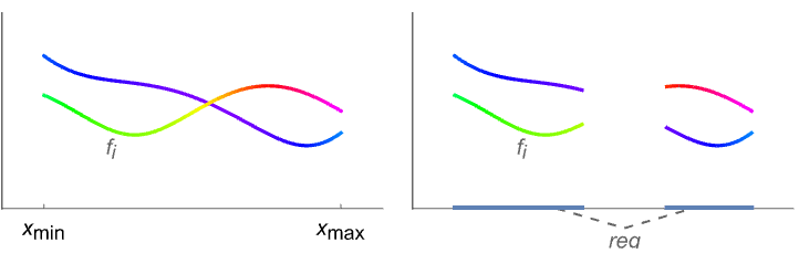
绘制几个函数.
AbsArgPlot[{…,w[fi],…},…]
绘制 fi,其特征由符号封装 w 定义.
AbsArgPlot[…,{x}∈reg]
变量 x 取自几何区域 reg.
AbsArgPlot
AbsArgPlot[f,{x,xmin,xmax}]
AbsArgPlot[{f1,f2,…},{x,xmin,xmax}]
绘制几个函数.
AbsArgPlot[{…,w[fi],…},…]
绘制 fi,其特征由符号封装 w 定义.
AbsArgPlot[…,{x}∈reg]
变量 x 取自几何区域 reg.
更多信息和选项
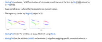
- AbsArgPlot 在不同的 x 值处计算 f,以创建形式为 {x,Abs[f[x]]} 的平滑曲线,并根据 {x,Arg[f[x]]} 着色.
- 在 fi 计算结果为非数字值的任何 x 处留下间断.
- 区域 reg 可为任意一维 RegionQ 对象.
- AbsArgPlot 将变量 x 视为局部变量,实际上相当于使用 Block.
- AbsArgPlot 具有属性 HoldAll,只在为 x 分配特定数值后才开始计算 f.
- 某些情况下,在将特定数值赋给 x 之前,通过 Evaluate 以符号方式对 f 进行计算可能更有效.
- 封装同时被应用于 Re[f] 和 Im[f].
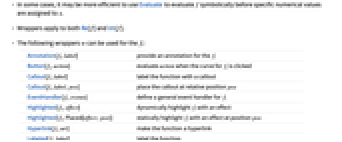
- 可对 fi 使用以下封装 w:
-
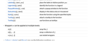
Annotation[fi,label] 为 fi 提供注释 Button[fi,action] 当点击 fi 曲线时,执行 action Callout[fi,label] 用 callout 标记函数 Callout[fi,label,pos] 把 callout 放在相对位置 pos EventHandler[fi,events] 为 fi 定义通用事件处理器 Highlighted[fi,effect] 用某种效果动态突出显示 fi Highlighted[fi,Placed[effect,pos]] 在位置 pos 处用某种效果静态突出显示 fi Hyperlink[fi,uri] 将函数变为超链接 Labeled[fi,label] 标记函数 Labeled[fi,label,pos] 把标签放在相对位置 pos Legended[fi,label] 在图例中标识函数 PopupWindow[fi,cont] 将弹出窗口附加到该函数 StatusArea[fi,label] 当鼠标移过时在状态栏中显示 Style[fi,styles] 用指定样式显示函数 Tooltip[fi,label] 为函数添加提示条 Tooltip[fi] 将函数用作提示条 - 可在多个层级上应用封装 w:
-
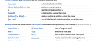
w[fi] 封装 fi w[{f1,…}] 封装一组 fi w1[w2[…]] 使用嵌套封装 - 在 Callout、Labeled 和 Placed 中可使用以下位置 pos:
-
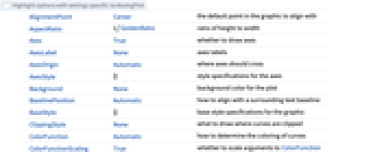
Automatic 自动放置标签 Above, Below, Before, After 曲线周围的位置 x 在位置 x 处的曲线周围 Scaled[s] 沿曲线的缩放过的位置 s {s,Above},{s,Below},… 沿曲线在位置 s 处的相对位置 {pos,epos} 在曲线的相对位置 pos 处放置的标签中的 epos - AbsArgPlot 具有与 Graphics 相同的选项,但有以下添加和更改: [所有选项的列表]
-
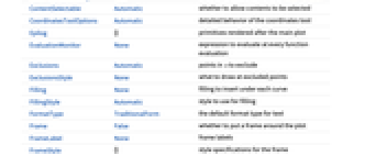
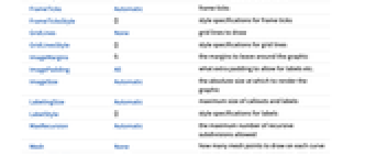
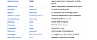
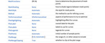
AspectRatio 1/GoldenRatio 高宽比 Axes True 是否绘制轴 ClippingStyle None 在曲线被剪裁的地方绘制什么 ColorFunction Automatic 如何确定曲线的颜色 ColorFunctionScaling True 是否将参数缩放到 ColorFunction EvaluationMonitor None 在每个函数求值时要计算的表达式 Exclusions Automatic x 中要排除的点 ExclusionsStyle None 在被排除点要绘制的内容 Filling None 填充以插入每条曲线下方 FillingStyle Automatic 用于填充的样式 LabelingSize Automatic 标注和标签的最大尺寸 MaxRecursion Automatic 允许的最大递归细分数量 Mesh None 在每条曲线上绘制网格点的数量 MeshFunctions {#1&} 如何确定网格点的位置 MeshShading None 如何对网格点之间的区域添加阴影 MeshStyle Automatic 网格点的样式 Method Automatic 用于优化曲线的方法 PerformanceGoal $PerformanceGoal 尝试优化的性能 PlotHighlighting Automatic 曲线的突出显示效果 PlotLabel None 绘图的整体标签 PlotLabels None 曲线使用的标签 PlotLegends None 曲线的图例 PlotPoints Automatic 初始样本点数量 PlotRange {Full,Automatic} 要包含的 y 或其他值的范围 PlotRangeClipping True 是否在绘图范围内裁剪 PlotStyle Automatic 用于指定每条曲线样式的图形指令 PlotTheme $PlotTheme 绘图的总体主题 RegionFunction (True&) 如何确定是否应包含某个点 ScalingFunctions None 如何缩放单个坐标 WorkingPrecision MachinePrecision 内部计算中使用的精度 - ClippingStyle 的可能设置有:
-

Automatic 用虚线显示剪掉的部分 

None 略去曲线被剪掉的部分 

style 用 style 显示剪掉的部分 - 在采用缺省设置 Exclusions->Automatic 和 ExclusionsStyle->None 的情况下,AbsArgPlot 将在检测出的断点和奇点处断开曲线. 设置为 Exclusions->None 时则在断点和奇点处连接曲线.
- Exclusions->{x1,x2,…} 等价于 Exclusions->{x==x1,x==x2,…}.
- PlotLabels->"Expressions" 用 fi 作为标记文字.
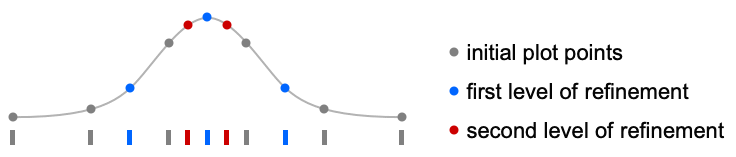
- 开始时,AbsArgPlot 会在 PlotPoints 指定的多个等间距的抽样点上计算 f. 然后使用自适应算法选择额外的抽样点,对给定区间进行最多 MaxRecursion 次分割.
- 因为只使用了有限数量的抽样点,AbsArgPlot 有可能会漏掉 f 的一些特征点. 增大 PlotPoints 和 MaxRecursion 的设置就可能捕捉到这些特征点.
- 影响曲线外观的主题包括:
-

"ThinLines" 细线 

"MediumLines" 中等粗细的线 

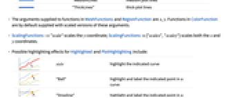
"ThickLines" 粗线 - 提供给 MeshFunctions 和 RegionFunction 中函数的参数为 x、y. 缺省情况下,为 ColorFunction 中的函数提供的是这些参数经过缩放的版本.
- ScalingFunctions->"scale" 缩放
坐标;ScalingFunctions{"scalex","scaley"} 同时缩放
和
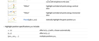
坐标. - Highlighted 和 PlotHighlighting 可用的突出显示效果包括:
-

style 突出显示指定的曲线 

"Ball" 突出显示并标注曲线上指定的点 
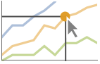
"Dropline" 突出显示并标注曲线上指定的点,同时绘制到坐标轴的准线 

"XSlice" 突出显示并标注垂直切片上的所有点 
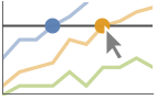
"YSlice" 突出显示并标注水平切片上的所有点 

Placed[effect,pos] 静态突出显示给定位置 pos - 突出显示的位置指定 pos 包括:
-
x, {x} 在 {x,y} 处突出显示,自动选择 y {x,y} 在 {x,y} 处突出显示 {pos1,pos2,…} 多个位置 posi
所有选项的列表
范例
打开所有单元 关闭所有单元基本范例 (6)
AbsArgPlot[Sin[I x] + Sin[Pi x], {x, -2, 2}]AbsArgPlot[{Sin[I x] + Sin[Pi x], 2Exp[I π x]}, {x, -2, 2}]AbsArgPlot[{Sin[I x] + Sin[Pi x], 2Exp[I π x]}, {x, -2, 2}, PlotLabels -> "Expressions"]AbsArgPlot[{Sin[I x] + Sin[Pi x], 2Exp[I π x]}, {x, -2, 2}, PlotLegends -> Automatic]AbsArgPlot[Sin[I x] + Sin[Pi x], {x, -2, 2}, Filling -> Axis]比较 Plot 和 AbsArgPlot:
{
{Plot[Abs[Sin[x] + Sin[I Sin[3x]]], {x, -Pi, Pi}], Plot[Arg[Sin[x] + Sin[I Sin[3x]]], {x, -Pi, Pi}, ColorFunction -> Hue]},
AbsArgPlot[Sin[x] + Sin[I Sin[3x]], {x, -Pi, Pi}]}范围 (18)
采样 (8)
AbsArgPlot[Sin[x] + Sin[I Sin[3x]], {x, 0, 4Pi}]AbsArgPlot[1 + Exp[-Abs[x]]Sin[I Sin[5x]], {x, -Pi, Pi}]AbsArgPlot[I + Floor[Sqrt[x]], {x, -100, 100}]用 Exclusions->None 绘制连续的曲线:
AbsArgPlot[I + Floor[Sqrt[x]], {x, -100, 100}, Exclusions -> None]用 PlotPoints 和 MaxRecursion 控制自适应采样:
Grid@Table[AbsArgPlot[Sin[I x] + Sin[Pi x], {x, -2, 2}, PlotPoints -> pp, MaxRecursion -> mr], {mr, {0, 1, 2}}, {pp, {15, 30}}]𝒟 = ImplicitRegion[-2 ≤ x ≤ 1 / 2∨1 ≤ x ≤ 2, {x}];AbsArgPlot[Sin[I x] + Sin[Pi x], {x}∈𝒟]用 MeshRegion 指定定义域:
𝒟 = MeshRegion[{{-2}, {-1}, {-1 / 2}, {1 / 2}, {1}, {2}}, Line[{{1, 2}, {3, 4}, {5, 6}}]];AbsArgPlot[Sin[x^2] - I, {x}∈𝒟]AbsArgPlot[{Sin[x] / x, 1 / x, -1 / x}, {x, -Infinity, Infinity}]添加标签和图例 (5)
AbsArgPlot[{ArcCos[x], ArcSin[x]}, {x, -3, 3}, PlotLegends -> Automatic]AbsArgPlot[{ArcCos[x], ArcSin[x]}, {x, -3, 3}, PlotLabels -> Automatic]AbsArgPlot[{Callout[ArcCos[x]], Tooltip[ArcSin[x]]}, {x, -3, 3}]AbsArgPlot[x^2 - 4, {x, -5, 5}]{AbsArgPlot[{x^2 - 4, Sinc[x]}, {x, -3, 3}, PlotHighlighting -> "Dropline"], AbsArgPlot[{x^2 - 4, Sinc[x]}, {x, -3, 3}, PlotHighlighting -> "XSlice"]}演示 (5)
AbsArgPlot[{ArcSin[x], ArcCos[x]}, {x, -3, 3}, PlotStyle -> {Thick, Dashed}]AbsArgPlot[{ArcSin[x], ArcCos[x]}, {x, -3, 3}, AxesLabel -> {x, ""}, PlotLabels -> Automatic, PlotLegends -> Automatic]AbsArgPlot[Sin[x] + Sin[I Sin[3x]], {x, -Pi, Pi}, Filling -> {1 -> Axis}]AbsArgPlot[{ArcSin[x], 3Exp[I x] + 0.5Exp[5I x]}, {x, -3, 3}, PlotTheme -> "Business"]用 ScalingFunctions 缩放坐标轴:
AbsArgPlot[x + I Exp[x], {x, -5, 5}, ScalingFunctions -> "Log"]选项 (113)
AspectRatio (4)
默认情况下,AbsArgPlot 使用固定不变的绘图的高宽比:
AbsArgPlot[x^2 - 4, {x, -4, 4}]通过 AspectRatio1 使高度和宽度一致:
AbsArgPlot[x^2 - 4, {x, -4, 4}, AspectRatio -> 1]AspectRatioAutomatic 则根据绘图的范围确定高宽比:
AbsArgPlot[x^2 - 4, {x, -4, 4}, AspectRatio -> Automatic]AspectRatioFull 调整高度和宽度,使图形正好可以放置在其他结构中:
plot = AbsArgPlot[x^2 - 4, {x, -4, 4}, AspectRatio -> Full];{Framed[Pane[plot, {50, 100}]], Framed[Pane[plot, {100, 100}]], Framed[Pane[plot, {100, 50}]]}Axes (4)
默认情况下,为 AbsArgPlot 绘制 Axes:
AbsArgPlot[x^2 - 4, {x, -4, 4}]使用 Frame 而非轴:
AbsArgPlot[x^2 - 4, {x, -4, 4}, Axes -> False, Frame -> True]使用 AxesOrigin 指定轴的相交处:
AbsArgPlot[x^2 - 4, {x, -4, 4}, AxesOrigin -> {0, 0}]{AbsArgPlot[x^2 - 4, {x, -4, 4}, Axes -> {True, False}], AbsArgPlot[x^2 - 4, {x, -4, 4}, Axes -> {False, True}]}AxesLabel (3)
AxesOrigin (2)
AxesStyle (4)
AbsArgPlot[x^2 - 4, {x, -4, 4}, AxesStyle -> Red]AbsArgPlot[x^2 - 4, {x, -4, 4}, AxesStyle -> {Directive[Thick, Brown], Directive[Thick, Blue]}]AbsArgPlot[x^2 - 4, {x, -4, 4}, AxesStyle -> Blue, TicksStyle -> Red]AbsArgPlot[x^2 - 4, {x, -4, 4}, AxesStyle -> Blue, LabelStyle -> Red]ClippingStyle (2)
ColorFunction (4)
AbsArgPlot[Sin[I x] + Sin[Pi x], {x, -2, 2}]AbsArgPlot[Sin[I x] + Sin[Pi x], {x, -2, 2}, ColorFunction -> "AvocadoColors"]ColorFunction 比 PlotStyle 的优先级高:
AbsArgPlot[Sin[I x] + Sin[Pi x], {x, -2, 2}, ColorFunction -> "AvocadoColors", PlotStyle -> Directive[Red, Dashed]]AbsArgPlot[Sin[I x] + Sin[Pi x], {x, -2, 2}, ColorFunction -> Function[{arg}, If[arg ≤ 0, Red, Green]], PlotStyle -> Thick, ColorFunctionScaling -> False]ColorFunctionScaling (1)
Exclusions (3)
ExclusionStyle (1)
Filling (4)
Table[AbsArgPlot[Sin[I x] + Sin[Pi x], {x, -3, 3}, Filling -> f], {f, {Axis, Top, Bottom, 3}}]AbsArgPlot[{Sin[I x] + Sin[Pi x], 2Exp[I π x]}, {x, -2, 2}, Filling -> Axis]AbsArgPlot[{ArcSin[x], 3Exp[I x] + 0.5Exp[5I x]}, {x, -3, 3}, Filling -> {1 -> Axis}]AbsArgPlot[{Sin[I x] + Sin[Pi x], 2Exp[I π x]}, {x, -2, 2}, Filling -> {1 -> {2}}]FillingStyle (2)
Table[AbsArgPlot[{ArcSin[x], 3Exp[I x] + 0.5Exp[5I x]}, {x, -3, 3}, Filling -> {1 -> Axis}, FillingStyle -> c], {c, {Red, Green, Blue, Yellow}}]在两条曲线间进行填充,在第二条曲线的下面用红色进行填充,上面则用蓝色:
AbsArgPlot[{ArcSin[x], Exp[I x] + 0.5Exp[5I x]}, {x, -3, 3}, Filling -> {1 -> {2}}, FillingStyle -> {Red, Blue}]Frame (3)
AbsArgPlot[x Sin[1 / x], {x, -.25, .25}, Frame -> True]AbsArgPlot[x Sin[1 / x], {x, -.25, .25}, Frame -> {{True, True}, {False, False}}]AbsArgPlot[x Sin[1 / x], {x, -.25, .25}, Frame -> {{False, False}, {True, True}}]FrameLabel (2)
FrameStyle (2)
AbsArgPlot[x Sin[1 / x], {x, -.25, .25}, Frame -> True, FrameStyle -> Directive[StandardBlue, Thick]]AbsArgPlot[x Sin[1 / x], {x, -.25, .25}, Frame -> True, FrameStyle -> {{Directive[Green, Thick], Directive[Red]}, {Directive[Gray, Thick], Directive[Blue]}}]FrameTicks (8)
默认情况下,自动放置 FrameTicks:
AbsArgPlot[x Sin[1 / x], {x, -.25, .25}, Frame -> True]AbsArgPlot[x Sin[1 / x], {x, -.25, .25}, Frame -> True, FrameTicks -> None]AbsArgPlot[x Sin[1 / x], {x, -.25, .25}, Frame -> True, FrameTicks -> {{False, False}, {True, True}}]AbsArgPlot[x Sin[1 / x], {x, -.25, .25}, Frame -> True, FrameTicks -> {{{0, .1, .2}, {0, .1, .2}}, {{-.2, .1, .2}, {-.2, .1, .2}}}]AbsArgPlot[x Sin[1 / x], {x, -.25, .25}, Frame -> True, FrameTicks -> {{{{0, a}, {.1, b}, {.2, c}}, {0, .1, .2}}, {{{-.2, -c}, {.1, b}, {.2, c}}, {-.2, .1, .2}}}]AbsArgPlot[x Sin[1 / x], {x, -.25, .25}, Frame -> True, FrameTicks -> {{{{0, a, .2}, {.1, b, .16}, {.2, c, .11}}, Automatic}, {Automatic, Automatic}}]AbsArgPlot[x Sin[1 / x], {x, -.25, .25}, Frame -> True, FrameTicks -> {{{{0, a, .2}, {.1, b, .16}, {.2, c, .11}}, {{0, a, {.2, 0}}, {.1, b, {.16, 0}}, {.2, c, {.11, 0}}}}, {Automatic, Automatic}}]AbsArgPlot[x Sin[1 / x], {x, -.25, .25}, Frame -> True, FrameTicks -> {{{{0, a, .2, Directive[Red]}, {.1, b, .16, Directive[Red, Thick, Dashed]}, {.2, c, .11, Directive[Red, Thick]}}, Automatic}, {Automatic, Automatic}}]minMeanMax[min_, max_] := {{min, min}, {(max + min) / 2, (max + min) / 2}, {max, max}}AbsArgPlot[x Sin[1 / x], {x, -.25, .25}, Frame -> True, FrameTicks -> {{Automatic, minMeanMax}, {Automatic, Automatic}}, PlotRangePadding -> None]FrameTicksStyle (3)
AbsArgPlot[x Sin[1 / x], {x, -.25, .25}, Frame -> True, Frame -> True, FrameStyle -> Directive[Red]]AbsArgPlot[x Sin[1 / x], {x, -.25, .25}, Frame -> True, Frame -> True, FrameTicks -> All, FrameTicksStyle -> {Directive[Green, Thick], Directive[Blue, Thick]}]AbsArgPlot[x Sin[1 / x], {x, -.25, .25}, Frame -> True, Frame -> True, FrameTicks -> All, FrameTicksStyle -> {{Gray, Blue}, {Red, Green}}]ImageSize (7)
使用有名称的尺寸如 Tiny、Small、Medium 和 Large:
{AbsArgPlot[x^2 - 4, {x, -4, 4}, ImageSize -> Tiny], AbsArgPlot[x^2 - 4, {x, -4, 4}, ImageSize -> Small]}{AbsArgPlot[x^2 - 4, {x, -4, 4}, ImageSize -> 150], AbsArgPlot[x^2 - 4, {x, -4, 4}, AspectRatio -> 1.5, ImageSize -> 150]}{AbsArgPlot[x^2 - 4, {x, -4, 4}, ImageSize -> {Automatic, 150}], AbsArgPlot[x^2 - 4, {x, -4, 4}, AspectRatio -> 2, ImageSize -> {Automatic, 150}]}{AbsArgPlot[x^2 - 4, {x, -4, 4}, ImageSize -> UpTo[200]], AbsArgPlot[x^2 - 4, {x, -4, 4}, AspectRatio -> 2, ImageSize -> UpTo[200]]}AbsArgPlot[x^2 - 4, {x, -4, 4}, ImageSize -> {200, 200}, Background -> StandardGray]设置 AspectRatioFull 将填充可用空间:
AbsArgPlot[x^2 - 4, {x, -4, 4}, AspectRatio -> Full, ImageSize -> {200, 200}, Background -> StandardGray]{AbsArgPlot[x^2 - 4, {x, -4, 4}, ImageSize -> {UpTo[150], UpTo[100]}], AbsArgPlot[x^2 - 4, {x, -4, 4}, AspectRatio -> 2, ImageSize -> {UpTo[150], UpTo[100]}]}设置 ImageSizeFull 将填充对象中的可用空间:
Framed[Pane[AbsArgPlot[x^2 - 4, {x, -4, 4}, ImageSize -> Full, Background -> StandardGray], {200, 100}]]Framed[Pane[AbsArgPlot[x^2 - 4, {x, -4, 4}, ImageSize -> {Scaled[0.5], Scaled[0.5]}, Background -> StandardGray], {200, 100}]]MaxRecursion (1)
每一级的 MaxRecursion 自适应地将初始网格细分为更精细的网格:
Table[AbsArgPlot[I + Sin[1 / x], {x, 0.001, .1}, MaxRecursion -> i, Mesh -> All, Ticks -> None], {i, {0, 3, 6}}]Mesh (3)
{AbsArgPlot[Cos[x] + I ArcCosh[x], {x, 0, 2Pi}, Mesh -> Full, MeshStyle -> AbsolutePointSize[3]], AbsArgPlot[Cos[x] + I ArcCosh[x], {x, 0, 2Pi}, Mesh -> All, MeshStyle -> AbsolutePointSize[3]]}AbsArgPlot[Cos[x] + I ArcCosh[x], {x, 0, 2Pi}, Mesh -> 10, MeshStyle -> AbsolutePointSize[5]]AbsArgPlot[Cos[x] + I ArcCosh[x], {x, 0, 2Pi}, Mesh -> {Range[0, 2Pi, Pi / 4]}, MeshStyle -> AbsolutePointSize[5], Ticks -> {Range[0, 2Pi, Pi / 4], Automatic}]MeshFunctions (2)
Table[AbsArgPlot[2Exp[I x] + 0.5Exp[3I x], {x, 0, 2Pi}, MeshFunctions -> {f}, Mesh -> 10, MeshStyle -> Black], {f, {Function[{x, y}, x], Function[{x, y}, y]}}]在
方向(黑色)上显示 10 个网格,在
方向(红色)显示 6 个网格:
AbsArgPlot[2Exp[I x] + 0.5Exp[3I x], {x, 0, 2Pi}, MeshFunctions -> {#1&, #2&}, Mesh -> {10, 6}, MeshStyle -> {Black, Red}]MeshShading (2)
AbsArgPlot[2Exp[I x] + 0.5Exp[3I x], {x, 0, 2Pi}, Mesh -> 15, MeshShading -> {None, Automatic}, MeshStyle -> Black]对于样式,MeshShading 比 PlotStyle 的优先级高:
AbsArgPlot[2Exp[I x] + 0.5Exp[3I x], {x, 0, 2Pi}, Mesh -> 15, MeshShading -> {None, Automatic}, MeshStyle -> Black, PlotStyle -> Directive[Black, Dashed]]MeshStyle (2)
AbsArgPlot[2Exp[I x] + 0.5Exp[3I x], {x, 0, 2Pi}, Mesh -> 10, MeshStyle -> Black]AbsArgPlot[2Exp[I x] + 0.5Exp[3I x], {x, 0, 2Pi}, Mesh -> 10, MeshFunctions -> {#1&, #2&}, MeshStyle -> {Directive[PointSize[Large], Black], Red}]PerformanceGoal (2)
PlotHighlighting (8)
当设置为 PlotHighlightingAutomatic 时,绘图有交互式坐标标注:
AbsArgPlot[Cos[x], {x, 0, 10}]用 PlotHighlightingNone 禁止整个绘图的突出显示:
AbsArgPlot[Cos[x], {x, 0, 10}, PlotHighlighting -> None]AbsArgPlot[E^Cos[x], {x, 0, 10}, PlotHighlighting -> "Ball"]AbsArgPlot[E^Cos[x] - 1, {x, 0, 10}, PlotHighlighting -> "Dropline"]AbsArgPlot[{E^Cos[x] - 1, Sin[x]}, {x, 0, 10}, PlotHighlighting -> "XSlice"]AbsArgPlot[E^Cos[x] - 1, {x, 0, 10}, PlotHighlighting -> "YSlice"]AbsArgPlot[{E^Cos[x] - 1, Sin[x]}, {x, 0, 10}, PlotHighlighting -> "XNearestPoint"]AbsArgPlot[{E^Cos[x] - 1, Sin[x]}, {x, 0, 10}, PlotHighlighting -> {"XNearestPoint", <|"Style" -> Green|>}]AbsArgPlot[{E^Cos[x] - 1, Sin[x]}, {x, 0, 10}, PlotHighlighting -> "XYLabel"]用 Callout 的选项改变标签的外观:
AbsArgPlot[E^Cos[x] - 1, {x, 0, 10}, PlotHighlighting -> {"XYLabel", <|"Appearance" -> "Corners", "CalloutMarker" -> "Circle"|>}]AbsArgPlot[E^Cos[x] - 1, {x, 0, 10}, PlotHighlighting -> {{"XNearestPoint", <|"Style" -> Black|>}, {"XYLabel", <|"Appearance" -> "Corners", "CalloutMarker" -> "Circle"|>}}]PlotLabel (1)
PlotLabels (6)
AbsArgPlot[{ArcSin[x], ArcCos[x]}, {x, -3, 3}, PlotLabels -> {"arcsine", "arccosine"}]AbsArgPlot[{ArcSin[x], ArcCos[x]}, {x, -3, 3}, PlotLabels -> Placed[{"arcsine", "arccosine"}, Above]]AbsArgPlot[{ArcSin[x], ArcCos[x]}, {x, -3, 3}, PlotLabels -> {Placed["arcsine", Below], Placed["arccosine", Above]}]PlotLabels->"Expressions" 将函数用作标签:
AbsArgPlot[{ArcSin[x], ArcCos[x]}, {x, -3, 3}, PlotLabels -> "Expressions"]AbsArgPlot[{ArcSin[x], ArcCos[x]}, {x, -3, 3}, PlotLabels -> {Callout["arcsine", Above], Callout["arccosine", Below]}]用 None 不添加标签:
AbsArgPlot[{ArcSin[x], ArcCos[x]}, {x, -3, 3}, PlotLabels -> {"arcsine", None}]PlotLegends (2)
PlotPoints (1)
PlotRange (1)
PlotStyle (2)
PlotTheme (1)
RegionFunction (1)
ScalingFunctions (6)
AbsArgPlot[x + I Exp[x], {x, -5, 5}]AbsArgPlot[x + I Exp[x], {x, -5, 5}, ScalingFunctions -> "Log"]AbsArgPlot[x + I Exp[x], {x, -5, 5}, ScalingFunctions -> {"Reverse", "Log"}]AbsArgPlot[Sinc[x], {x, -Infinity, Infinity}]AbsArgPlot[Sinc[x], {x, 0, Infinity}, ScalingFunctions -> {"Reverse", None}]使用 Interval 关注无限域中需要注意的区域:
AbsArgPlot[x ^ 2 * Sin[1 / x], {x, -Infinity, Infinity}, ScalingFunctions -> {{"Infinite", Interval[{-1, 1}]}, None}]Ticks (9)
AbsArgPlot[x Sin[1 / x], {x, -.25, .25}]AbsArgPlot[x Sin[1 / x], {x, -.25, .25}, Axes -> True, Ticks -> None]AbsArgPlot[x Sin[1 / x], {x, -.25, .25}, Axes -> True, Ticks -> {Automatic, None}]AbsArgPlot[x Sin[1 / x], {x, -.25, .25}, Axes -> True, Ticks -> {{-.2, .1, .2}, {0, .1, .2}}]AbsArgPlot[x Sin[1 / x], {x, -.25, .25}, Axes -> True, Ticks -> {{{-.2, "-a"}, {.1, "b"}, {.2, "a"}}, {{0, 0}, {.1, "c"}, {.2, "d"}}}]AbsArgPlot[x Sin[1 / x], {x, -.25, .25}, Axes -> True, Ticks -> {{{-.2, "-a"}, {.1, "b"}, {.2, "a"}}, Automatic}]AbsArgPlot[x Sin[1 / x], {x, -.25, .25}, Axes -> True, Ticks -> {{{-.2, "-a", .05}, {.1, "b", .05}, {.2, "a", .05}}, {{0, "-d", .05}, {.13, "c", .25}, {.2, "d", .4}}}]AbsArgPlot[x Sin[1 / x], {x, -.25, .25}, Axes -> True, Ticks -> {{{-.2, "-a", .05}, {.1, "b", {.05, .1}}, {.2, "a", .05}}, {{0, "-d", .05}, {.13, "c", {.25, .1}}, {.2, "d", {.4, .1}}}}]AbsArgPlot[x Sin[1 / x], {x, -.25, .25}, Axes -> True, Ticks -> {{{-.2, "-a", .05, Directive[Red]}, {.1, "b", .05, Directive[Orange]}, {.2, "a", .15, Directive[Thick, Orange]}}, {{0, "-d", .05}, {.13, "c", .25, Directive[Thick, Green]}, {.21, "d", .42, Directive[Blue]}}}]minMeanMax[min_, max_] := {{min, min}, {(max + min) / 2, (max + min) / 2}, {max, max}}AbsArgPlot[x Sin[1 / x], {x, -.25, .25}, Axes -> True, Ticks -> {Automatic, minMeanMax}]TicksStyle (4)
AbsArgPlot[x Sin[1 / x], {x, -.25, .25}, Axes -> True, AxesStyle -> Red]AbsArgPlot[x Sin[1 / x], {x, -.25, .25}, Axes -> True, TicksStyle -> Directive[Red]]AbsArgPlot[x Sin[1 / x], {x, -.25, .25}, TicksStyle -> {Directive[Red], Directive[Blue]}]AbsArgPlot[x Sin[1 / x], {x, -.25, .25}, TicksStyle -> Directive[Red, Thick], LabelStyle -> Blue]应用 (3)
f1 = Exp[-x^2]UnitStep[x];
f2 = Exp[-x^2](UnitStep[x + 1] - UnitStep[x - 2]);
ft1 = FourierTransform[f1, x, k];
ft2 = FourierTransform[f2, x, k];AbsArgPlot[{ft1, ft2}, {k, -20, 20}, PlotRange -> All, ScalingFunctions -> "Log", PlotLabels -> {ℱ[f1], ℱ[f2]}]sol = NDSolve[{y''[x] - I Sin[y[x]] / 2 == 0, y[0] == 2, y'[0] == I}, y[x], {x, 0, 60}][[1]];AbsArgPlot[Evaluate[y[x] /. sol], {x, 0, 60}, PlotRange -> All, ColorFunction -> (Hue[(#/Pi)]&), ColorFunctionScaling -> False, PlotLegends -> Automatic]AbsArgPlot[EllipticE[x], {x, -5, 5}, Exclusions -> None, PlotLegends -> Automatic]属性和关系 (8)
AbsArgPlot 是 Plot 的一种特殊情况:
{Plot[Abs[ArcSin[x]], {x, -3, 3}], AbsArgPlot[ArcSin[x], {x, -3, 3}]}ComplexPlot 使用颜色表示函数的自变量和幅值:
ComplexPlot[Log[z], {z, 3}]使用 ComplexPlot3D 使用
轴表示幅值:
ComplexPlot3D[Log[z], {z, 3}]使用 ReImPlot 在实数上绘制实部和虚部:
ReImPlot[Log[x], {x, -3, 3}]使用 ComplexListPlot 显示复数在平面中的位置:
ComplexListPlot[RandomComplex[{-3 - 3I, 3 + 3I}, 100]]ComplexContourPlot 绘制复数曲线:
ComplexContourPlot[Abs[Log[z]] == 1, {z, 3}]ComplexRegionPlot 绘制复数区域:
ComplexRegionPlot[Abs[Log[z]] < 1, {z, 3}]ComplexStreamPlot 和 ComplexVectorPlot 将复数视作方向:
ComplexStreamPlot[Log[z], {z, 3}]ComplexVectorPlot[Log[z], {z, 3}]可能存在的问题 (2)
AbsArgPlot[x + (-2^x + 1 - I / 10 - x)UnitStep[x], {x, -1, 1}, PlotLegends -> Automatic]{AbsArgPlot[Exp[I x], {x, 0, 2Pi}, Mesh -> 15, MeshStyle -> Black], AbsArgPlot[Exp[I x], {x, 0, 2Pi}, Mesh -> 15, MeshStyle -> Black, Exclusions -> None]}文本
Wolfram Research (2019),AbsArgPlot,Wolfram 语言函数,https://reference.wolfram.com/language/ref/AbsArgPlot.html (更新于 2023 年).
CMS
Wolfram 语言. 2019. "AbsArgPlot." Wolfram 语言与系统参考资料中心. Wolfram Research. 最新版本 2023. https://reference.wolfram.com/language/ref/AbsArgPlot.html.
APA
Wolfram 语言. (2019). AbsArgPlot. Wolfram 语言与系统参考资料中心. 追溯自 https://reference.wolfram.com/language/ref/AbsArgPlot.html 年
BibTeX
@misc{reference.wolfram_2026_absargplot, author="Wolfram Research", title="{AbsArgPlot}", year="2023", howpublished="\url{https://reference.wolfram.com/language/ref/AbsArgPlot.html}", note=[Accessed: 05-September-2026]}
BibLaTeX
@online{reference.wolfram_2026_absargplot, organization={Wolfram Research}, title={AbsArgPlot}, year={2023}, url={https://reference.wolfram.com/language/ref/AbsArgPlot.html}, note=[Accessed: 05-September-2026]}