


GraphPlot3D
GraphPlot3D[g]
generates a 3D plot of the graph g.
GraphPlot3D[{e1,e2,…}]
generates a 3D plot of the graph with edges ei.
GraphPlot3D[{…,w[ei],…}]
plots ei with features defined by the symbolic wrapper w.
GraphPlot3D[{vi 1vj 1,…}]
uses rules vikvjk to specify the graph g.
GraphPlot3D[m]
uses the adjacency matrix m to specify the graph g.
Details and Options
- GraphPlot3D attempts to place vertices in 3D to give a well-laid-out version of the graph.
- GraphPlot3D supports the same vertices, edges and wrappers as Graph.
- The following special wrappers can be used for the edges ei:
-
Annotation[ei,label] provide an annotation Button[ei,action] define an action to execute when the element is clicked EventHandler[ei,…] define a general event handler for the element Hyperlink[ei,uri] make the element act as a hyperlink Labeled[ei,…] display the element with labeling PopupWindow[ei,cont] attach a popup window to the element StatusArea[ei,label] display in the status area when the element is moused over Style[ei,opts] show the element using the specified styles Tooltip[ei,label] attach an arbitrary tooltip to the element - GraphPlot3D has the same options as Graphics3D, with the following additions and changes: [List of all options]
-
DataRange Automatic the range of vertex coordinates to generate DirectedEdges False whether to interpret Rule as DirectedEdge EdgeLabels None labels and placements for edges EdgeLabelStyle Automatic style to use for edge labels EdgeShapeFunction Automatic generate graphic shapes for edges EdgeStyle Automatic styles for edges GraphLayout Automatic how to lay out vertices and edges GraphHighlight {} vertices and edges to highlight GraphHighlightStyle Automatic style for highlight Method Automatic method to use PerformanceGoal Automatic aspects of performance to try to optimize PlotStyle Automatic graphics directives to determine styles PlotTheme Automatic overall theme for the graph VertexCoordinates Automatic coordinates for vertices VertexLabels None labels and placements for vertices VertexLabelStyle Automatic style to use for vertex labels VertexShape Automatic graphic shape for vertices VertexShapeFunction Automatic generate graphic shapes for vertices VertexSize Automatic size of vertices VertexStyle Automatic styles for vertices - With the setting VertexCoordinates->Automatic, the embedding of vertices and routing of edges is computed automatically, based on the setting for GraphLayout.
- Possible special embeddings for GraphLayout include:
-

"BipartiteEmbedding" vertices on two parallel lines 
"CircularEmbedding" vertices on a circle 
"CircularMultipartiteEmbedding" vertices on segments of a circle 
"DiscreteSpiralEmbedding" vertices on a discrete spiral 
"GridEmbedding" vertices on a grid 
"LinearEmbedding" vertices on a line 
"MultipartiteEmbedding" vertices on several parallel lines 
"SpiralEmbedding" vertices on a 3D spiral projected to 2D 
"StarEmbedding" vertices on a circle with a center - Possible structured embeddings for layered graphs such as trees and directed acyclic graphs include:
-

"BalloonEmbedding" vertices on a circle with the center at the parent vertex 
"RadialEmbedding" vertices on a circular segment 
"LayeredDigraphEmbedding" vertices on parallel lines for directed acyclic graphs 
"LayeredEmbedding" vertices on parallel lines - Possible optimizing embeddings all minimize a quantity and include:
-

"HighDimensionalEmbedding" energy for spring-electrical in high dimension 
"PlanarEmbedding" number of edge crossings 
"SpectralEmbedding" weighted sum of squares distances 
"SpringElectricalEmbedding" energy with edges as springs and vertices as charges 
"SpringEmbedding" energy with edges as springs 
"TutteEmbedding" number of edge crossings and distance to neighbors - Possible settings for PlotTheme include common base themes, color feature themes, font features themes, and size features themes.
-
"Business" a bright, modern look appropriate for business presentations or infographics 
"Detailed" identify data by employing labels and tooltips 
"Marketing" elegant, eye-catching design suitable for marketing needs 
"Minimal" simple graph 
"Monochrome" single-color design 
"Scientific" candid design useful for analyzing detailed data with labels and tooltips 
"Web" clean, bold design suitable for a consumer website or blog 
"Classic" historical design of graph to remain compatible with existing uses - Graph features themes affect plot of vertices and edges. Feature themes include:
-
"LargeGraph" large graph 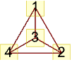
"ClassicLabeled" classic graph 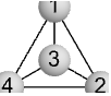
"IndexLabeled" index-labeled graph
List of all options
Examples
open all close allBasic Examples (3)
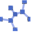
GraphPlot3D[ButterflyGraph[2]]Plot a graph specified by edge rules:
GraphPlot3D[{1 -> 2, 2 -> 3, 3 -> 4, 4 -> 1, 4 -> 5, 5 -> 1, 2 -> 5, 3 -> 5}]Plot a graph specified by its adjacency matrix:
GraphPlot3D[{{0, 1, 1, 1}, {1, 0, 1, 1}, {1, 1, 0, 1}, {1, 1, 1, 0}}]Scope (12)
Graph Specification (6)
Specify a graph using a graph:
GraphPlot3D[Graph[{12, 23, 34, 41, 24}]]Specify a graph using a rule list:
GraphPlot3D[{1 -> 2, 2 -> 3, 3 -> 4, 4 -> 1, 2 -> 4}]Specify a graph using a dense adjacency matrix:
GraphPlot3D[{{0, 1, 0, 0}, {0, 0, 1, 1}, {0, 0, 0, 1}, {1, 0, 0, 0}}]Specify a graph using a sparse adjacency matrix:
GraphPlot3D[SparseArray[{{1, 2}, {2, 3}, {3, 4}, {4, 1}, {2, 4}} -> 1, {4, 4}]]Use GraphData for collections of graphs:
Table[GraphPlot3D[GraphData[g, "EdgeRules"]], {g, {{"GeneralizedPetersen", {9, 2}}, "ClebschGraph", "TesseractGraph"}}]Use ExampleData for collections of sparse matrices:
GraphPlot3D[ExampleData[{"Matrix", "Bai/dwa512"}, "Matrix"]]Graph Styling (6)
GraphPlot3D[{1 -> 2, Labeled[2 -> 3, "23"], 3 -> 1, 2 -> 4, 2 -> 5}]GraphPlot3D[{5 -> 4, 6 -> 2, 6 -> 3, 6 -> 5, 4 -> 5, 7 -> 1, 7 -> 3, 7 -> 4, 7 -> 6}, VertexLabels -> "Name"]GraphPlot3D[{1 -> 2, 2 -> 3, 3 -> 1}, DirectedEdges -> True]Plot a disconnected graph using different packing methods:
Table[Framed@GraphPlot3D[Table[i -> Mod[i ^ 2, 102], {i, 0, 102}], GraphLayout -> {"PackingLayout" -> pm}], {pm, {Automatic, "ClosestPacking"}}]For very large graphs, it is often better not to draw vertices at all:
GraphPlot3D[Table[i -> Mod[i ^ 2, 500], {i, 500}], VertexShapeFunction -> None]Use EdgeShapeFunction and VertexShapeFunction for detailed control:
GraphPlot3D[{1 -> 2, 2 -> 3, 3 -> 4, 4 -> 1, 4 -> 5, 5 -> 1, 2 -> 5, 3 -> 5}, EdgeShapeFunction -> (Cylinder[#1, .05]&), VertexShapeFunction -> (Sphere[#1, .1]&)]Options (90)
Axes (3)
By default, Axes are not drawn:
GraphPlot3D[ButterflyGraph[3]]Use AxesTrue to turn on axes:
GraphPlot3D[ButterflyGraph[3], Axes -> True]Turn each axis on individually:
{GraphPlot3D[ButterflyGraph[3], Axes -> {True, False, False}], GraphPlot3D[ButterflyGraph[3], Axes -> {False, True, False}], GraphPlot3D[ButterflyGraph[3], Axes -> {False, False, True}]}AxesLabel (3)
AxesOrigin (2)
AxesStyle (4)
Change the style for the axes:
GraphPlot3D[ButterflyGraph[3], Axes -> True, AxesStyle -> Red]Specify the style of each axis:
GraphPlot3D[ButterflyGraph[3], Axes -> True, AxesStyle -> {{Thick, Brown}, {Thick, Blue}, {Thick, Green}}]Use different styles for the ticks and the axes:
GraphPlot3D[ButterflyGraph[3], Axes -> True, AxesStyle -> Green, TicksStyle -> Red]Use different styles for the labels and the axes:
GraphPlot3D[ButterflyGraph[3], Axes -> True, AxesStyle -> Green, LabelStyle -> Red]DataRange (1)
DirectedEdges (1)
GraphLayout (66)
"BalloonEmbedding" (6)
Place each vertex in an enclosing circle centered at its parent vertex:
GraphPlot3D[Table[Floor[j / 12]j, {j, 1, 30}], GraphLayout -> "BalloonEmbedding"]"BalloonEmbedding" works best for tree graphs:
GraphPlot3D[RandomInteger[{1, #}] # + 1 & /@ Range[30], GraphLayout -> "BalloonEmbedding"]Use the option "EvenAngle"->True to place vertices evenly in an enclosing circle:
GraphPlot3D[KaryTree[48, 5], GraphLayout -> {"BalloonEmbedding", "EvenAngle" -> #}]& /@ {True, False}With the setting "OptimalOrder"->True, the vertex ordering optimizes the angular resolution and the aspect ratio:
GraphPlot3D[KaryTree[48, 5], GraphLayout -> {"BalloonEmbedding", "OptimalOrder" -> #}]& /@ {True, False}Use the option "RootVertex"->v to set the root vertex:
GraphPlot3D[KaryTree[48, 5], GraphLayout -> {"BalloonEmbedding", "RootVertex" -> #}]& /@ {1, 2}Use "SectorAngles"->s to control the size of each sector:
GraphPlot3D[KaryTree[48, 5], GraphLayout -> {"BalloonEmbedding", "SectorAngles" -> {1 -> Pi / 2}}]"BipartiteEmbedding" (1)
"CircularEmbedding" (2)
GraphPlot3D[Table[iMod[i + 1, 3], {i, 8}], GraphLayout -> "CircularEmbedding"]Use the option "Offset"->offset to specify the offset angles:
GraphPlot3D[CompleteGraph[7], GraphLayout -> {"CircularEmbedding", "Offset" -> #}]& /@ {Automatic, {30 Degree, 30 Degree}, {50 Degree, 80 Degree}}"CircularMultipartiteEmbedding" (2)
Place vertices on polygon lines based on a vertex partition:
GraphPlot3D[Flatten[Table[ij, {i, 4}, {j, 5, 8}]], GraphLayout -> {"CircularMultipartiteEmbedding", "VertexPartition" -> {2, 3, 3}}]Use "VertexPartition"->partition to specify a partition of vertices:
GraphPlot3D[CompleteGraph[{3, 3, 2}], GraphLayout -> {"CircularMultipartiteEmbedding", "VertexPartition" -> {3, 3, 2}}]"DiscreteSpiralEmbedding" (3)
Place vertices on a discrete spiral:
GraphPlot3D[Table[ii + 1, {i, 11}], GraphLayout -> "DiscreteSpiralEmbedding"]"DiscreteSpiralEmbedding" works best for path graphs:
GraphPlot3D[PathGraph[Range[30]], GraphLayout -> "DiscreteSpiralEmbedding"]With the setting "OptimalOrder"True, vertices are reordered so that they lie nicely on a discrete spiral:
edges = RandomSample[EdgeList[PathGraph[Range[20]]], 19];
{GraphPlot3D[edges, GraphLayout -> {"DiscreteSpiralEmbedding", "OptimalOrder" -> True}],
	GraphPlot3D[edges, GraphLayout -> {"DiscreteSpiralEmbedding", "OptimalOrder" -> False}]}
"GridEmbedding" (2)
"HighDimensionalEmbedding" (2)
Place vertices in high dimension according to spring-electrical embedding and project down:
GraphPlot3D[{12, 13, 15, 19, 24, 26, 210, 34, 37, 311, 48, 412, 56, 57, 513, 68, 614, 78, 715, 816, 910, 911, 913, 1012, 1014, 1112, 1115, 1216, 1314, 1315, 1416, 1516}, GraphLayout -> "HighDimensionalEmbedding"]Use "RandomSeed"->int to specify a seed for the random number generator that computes the initial vertex placement:
edge = {13, 15, 17, 23, 26, 27, 28, 34, 38, 46, 58, 78};GraphPlot3D[edge, GraphLayout -> {"HighDimensionalEmbedding", "RandomSeed" -> #}]& /@ {1, 50}"LayeredEmbedding" (6)
Place vertices in several layers in such a way as to minimize edges between nonadjacent layers:
GraphPlot3D[Table[iMod[i + 1, 5], {i, 12}], GraphLayout -> "LayeredEmbedding"]"LayeredEmbedding" works best for tree graphs:
GraphPlot3D[RandomInteger[{1, #}] # + 1 & /@ Range[20], GraphLayout -> "LayeredEmbedding"]Use the option "LayerSizeFunction"->func to specify the relative height:
GraphPlot3D[KaryTree[10, 3], GraphLayout -> {"LayeredEmbedding", LayerSizeFunction -> (2&)}]Use the option "RootVertex"->v to set the root vertex:
GraphPlot3D[KaryTree[10, 3], GraphLayout -> {"LayeredEmbedding", "RootVertex" -> #}]& /@ {1, 4}Use the option "LeafDistance"->d to specify the leaf distance:
GraphPlot3D[KaryTree[10, 3], GraphLayout -> {"LayeredEmbedding", "LeafDistance" -> #}]& /@ {1, 2}Use the option "Orientation"->o to draw a tree with different orientations:
Table[GraphPlot3D[KaryTree[6, 3], GraphLayout -> {"LayeredEmbedding", "Orientation" -> o}], {o, {Top, Bottom, Left, Right}}]"LayeredDigraphEmbedding" (3)
Place vertices in a series of layers:
GraphPlot3D[{12, 13, 23, 14, 24, 15}, GraphLayout -> "LayeredDigraphEmbedding"]Use the option "RootVertex"->v to set the root vertex:
GraphPlot3D[{12, 13, 23, 14, 24, 15}, GraphLayout -> {"LayeredDigraphEmbedding", "RootVertex" -> #}]& /@ {1, 3}Use the option "Orientation"->o to draw a tree with different orientations:
Table[GraphPlot3D[{12, 13, 23, 14, 24, 15}, GraphLayout -> {"LayeredDigraphEmbedding", "Orientation" -> o}], {o, {Top, Bottom, Left, Right}}]"LinearEmbedding" (2)
GraphPlot3D[{12, 23, 34}, GraphLayout -> "LinearEmbedding"]Use the option "Method"->m to specify the algorithm:
Table[GraphPlot3D[CompleteGraph[4], GraphLayout -> {"LinearEmbedding", Method -> m}], {m, {"Spectral", "SpectralOrdering", "TwoNormApproximation", "TwoNormApproximationOrdering"}}]"MultipartiteEmbedding" (2)
Place vertices on multiple line grids based on a vertex partition:
GraphPlot3D[Flatten[Table[ij, {i, 3}, {j, 4, 8}]], GraphLayout -> {"MultipartiteEmbedding", "VertexPartition" -> {2, 1, 3, 2}}]Use "VertexPartition"->partition to specify a partition of vertices:
GraphPlot3D[CompleteGraph[{3, 2, 4}], GraphLayout -> {"MultipartiteEmbedding", "VertexPartition" -> {3, 2, 4}}]"PlanarEmbedding" (1)
"RadialEmbedding" (2)
Place vertices in concentric circles:
GraphPlot3D[Table[Floor[j / 7]j, {j, 1, 30}], GraphLayout -> "RadialEmbedding"]Use the option "RootVertex"->v to set the root vertex:
GraphPlot3D[KaryTree[60, 5], GraphLayout -> {"RadialEmbedding", "RootVertex" -> #}]& /@ {1, 2}"RandomEmbedding" (1)
"SpectralEmbedding" (2)
Place vertices so the weighted sum of squares of mutual distances is minimized:
GraphPlot3D[{12, 13, 15, 19, 24, 26, 210, 34, 37, 311, 48, 412, 56, 57, 513, 68, 614, 78, 715, 816, 910, 911, 913, 1012, 1014, 1112, 1115, 1216, 1314, 1315, 1416, 1516}, GraphLayout -> "SpectralEmbedding"]Use the option "RelaxationFactor"->r to get the layout based on a relaxed Laplace matrix.
Table[GraphPlot3D[GridGraph[{10, 10}], GraphLayout -> {"SpectralEmbedding", "RelaxationFactor" -> i}], {i, 0, 1, .3}]"SpiralEmbedding" (2)
GraphPlot3D[Table[iMod[i + 1, 20, 1], {i, 20}], GraphLayout -> "SpiralEmbedding"]With the setting "OptimalOrder"->True, vertices are reordered so that they lie on the spiral nicely:
edges = RandomSample[EdgeList[CycleGraph[20]], 20];
GraphPlot3D[edges, GraphLayout -> {"SpiralEmbedding", "OptimalOrder" -> #}]& /@ {True, False}
"SpringElectricalEmbedding" (12)
Place vertices so that they minimize mechanical and electrical energy when each vertex has a charge and each edge corresponds to a spring:
GraphPlot3D[{12, 13, 15, 19, 24, 26, 210, 34, 37, 311, 48, 412, 56, 57, 513, 68, 614, 78, 715, 816, 910, 911, 913, 1012, 1014, 1112, 1115, 1216, 1314, 1315, 1416, 1516}, GraphLayout -> "SpringElectricalEmbedding"]With the setting "EdgeWeighted"->True, edge weights are used:
edge = RandomInteger[#]# + 1& /@ Range[0, 10];
weight = RandomInteger[{1, 5}, 11];GraphPlot3D[edge, EdgeWeight -> weight, GraphLayout -> {"SpringElectricalEmbedding", "EdgeWeighted" -> #}]& /@ {True, False}Use the option "EnergyControl"->e to specify limitations on the total energy of the system during minimization:
edge = RandomInteger[#]# + 1& /@ Range[0, 20];GraphPlot3D[edge, {GraphLayout -> {"SpringElectricalEmbedding", "EnergyControl" -> #, "StepControl" -> "Monotonic"}}]& /@ {Automatic, "Monotonic", "NonMonotonic"}Use "InferentialDistance"->d to specify a cutoff distance beyond which the interaction between vertices is assumed to be nonexistent:
edge = RandomInteger[#]# + 1& /@ Range[0, 20];GraphPlot3D[edge, GraphLayout -> {"SpringElectricalEmbedding", "InferentialDistance" -> #}]& /@ {Automatic, .1, .5}Use "MaxIteration"->it to specify a maximum number of iterations to be used in attempting to minimize the energy:
edge = RandomInteger[#]# + 1& /@ Range[0, 20];GraphPlot3D[edge, GraphLayout -> {"SpringElectricalEmbedding", "MaxIteration" -> #}]& /@ {Automatic, 1, 2}Use "Multilevel"->method to specify a method used during a recursive procedure of coarsening a graph:
edge = RandomInteger[#]# + 1& /@ Range[0, 20];GraphPlot3D[edge, GraphLayout -> {"SpringElectricalEmbedding", "Multilevel" -> #}]& /@ {Automatic, None, "MaximalIndependentVertexSet", "MaximalIndependentVertexSetRugeStuben", "MaximalIndependentVertexSetInjection", "MaximalIndependentVertexSetRugeStubenInjection", "MaximalIndependentEdgeSetHeavyEdge", "MaximalIndependentEdgeSet", "MaximalIndependentEdgeSetSmallestVertexWeight", "Hybrid"}With the setting "Octree"->True, an octree data structure (in three dimensions) or a quadtree data structure (in two dimensions) is used in the calculation of repulsive force:
edge = RandomInteger[#]# + 1& /@ Range[0, 20];GraphPlot3D[edge, GraphLayout -> {"SpringElectricalEmbedding", "Octree" -> #}]& /@ {True, False}Use "RandomSeed"->int to specify a seed for the random number generator that computes the initial vertex placement:
edge = RandomInteger[#]# + 1& /@ Range[0, 20];GraphPlot3D[edge, GraphLayout -> {"SpringElectricalEmbedding", "RandomSeed" -> #}]& /@ {1, 5}Use "RepulsiveForcePower"->r to control how fast the repulsive force decays over distance:
edge = RandomInteger[#]# + 1& /@ Range[0, 20];GraphPlot3D[edge, GraphLayout -> {"SpringElectricalEmbedding", "RepulsiveForcePower" -> #}]& /@ {-1, -2.5}Use "StepControl"->method to define how step length is modified during energy minimization:
edge = RandomInteger[#]# + 1& /@ Range[0, 20];GraphPlot3D[edge, GraphLayout -> {"SpringElectricalEmbedding", "StepControl" -> #}]& /@ {Automatic, "Monotonic", "NonMonotonic", "StrictlyMonotonic"}Use "StepLength"->r to specify the initial step length used in moving the vertices around:
edge = RandomInteger[#]# + 1& /@ Range[0, 20];GraphPlot3D[edge, GraphLayout -> {"SpringElectricalEmbedding", "StepLength" -> #}]& /@ {1, 4.5}Use "Tolerance"->r to specify the tolerance used in terminating the energy minimization process:
edge = RandomInteger[#]# + 1& /@ Range[0, 20];GraphPlot3D[edge, GraphLayout -> {"SpringElectricalEmbedding", "Tolerance" -> #}]& /@ {Automatic, .5}"SpringEmbedding" (10)
Place vertices so that they minimize mechanical energy when each edge corresponds to a spring:
GraphPlot3D[{114, 115, 116, 25, 26, 213, 37, 314, 319, 48, 415, 420, 511, 519, 612, 620, 711, 716, 812, 816, 910, 914, 917, 1015, 1018, 1112, 1317, 1318, 1719, 1820}, GraphLayout -> "SpringEmbedding"]With the setting "EdgeWeighted"->True, edge weights are used:
edge = RandomInteger[#]# + 1& /@ Range[0, 10];
weight = RandomInteger[{1, 5}, 11];GraphPlot3D[edge, EdgeWeight -> weight, GraphLayout -> {"SpringEmbedding", "EdgeWeighted" -> #}]& /@ {True, False}Use the option "EnergyControl"->e to specify limitations on the total energy of the system during minimization:
edge = RandomInteger[#]# + 1& /@ Range[0, 30];GraphPlot3D[edge, {GraphLayout -> {"SpringEmbedding", "EnergyControl" -> #}}]& /@ {Automatic, "Monotonic", "NonMonotonic"}Use "InferentialDistance"->d to specify a cutoff distance beyond which the interaction between vertices is assumed to be nonexistent:
edge = RandomInteger[#]# + 1& /@ Range[0, 30];GraphPlot3D[edge, GraphLayout -> {"SpringEmbedding", "InferentialDistance" -> #}]& /@ {Automatic, .5, 2}Use "MaxIteration"->it to specify a maximum number of iterations to be used in attempting to minimize the energy:
edge = RandomInteger[#]# + 1& /@ Range[0, 30];GraphPlot3D[edge, GraphLayout -> {"SpringEmbedding", "MaxIteration" -> #}]& /@ {Automatic, 1, 2}Use "Multilevel"->method to specify a method used during a recursive procedure of coarsening a graph:
edge = RandomInteger[#]# + 1& /@ Range[0, 30];GraphPlot3D[edge, GraphLayout -> {"SpringEmbedding", "Multilevel" -> #}]& /@ {Automatic, None, "MaximalIndependentVertexSet", "MaximalIndependentVertexSetRugeStuben", "MaximalIndependentVertexSetInjection", "MaximalIndependentVertexSetRugeStubenInjection", "MaximalIndependentEdgeSetHeavyEdge", "MaximalIndependentEdgeSet", "MaximalIndependentEdgeSetSmallestVertexWeight", "Hybrid"}Use "RandomSeed"->int to specify a seed for the random number generator that computes the initial vertex placement:
edge = RandomInteger[#]# + 1& /@ Range[0, 30];GraphPlot3D[edge, GraphLayout -> {"SpringEmbedding", "RandomSeed" -> #}]& /@ {1, 5}Use "StepControl"->method to define how step length is modified during energy minimization:
edge = RandomInteger[#]# + 1& /@ Range[0, 30];GraphPlot3D[edge, GraphLayout -> {"SpringEmbedding", "StepControl" -> #}]& /@ {Automatic, "Monotonic", "NonMonotonic", "StrictlyMonotonic"}Use "StepLength"->r to specify the initial step length used in moving the vertices around:
edge = RandomInteger[#]# + 1& /@ Range[0, 30];GraphPlot3D[edge, GraphLayout -> {"SpringEmbedding", "StepLength" -> #}]& /@ {1, 4.5}Use "Tolerance"->r to specify the tolerance used in terminating the energy minimization process:
edge = RandomInteger[#]# + 1& /@ Range[0, 30];GraphPlot3D[edge, GraphLayout -> {"SpringEmbedding", "Tolerance" -> #}]& /@ {Automatic, .5}"StarEmbedding" (3)
Place vertices on a star shape:
GraphPlot3D[Table[1i, {i, 2, 6}], GraphLayout -> "StarEmbedding"]Use the option "Offset"->offset to specify the offset angles:
GraphPlot3D[StarGraph[15], GraphLayout -> {"StarEmbedding", "Offset" -> #}]& /@ {Automatic, {30 Degree, 30 Degree}, {50 Degree, 80 Degree}}Use the option "Center"->center to specify the center:
GraphPlot3D[StarGraph[15], GraphLayout -> {"StarEmbedding", "Center" -> #}]& /@ {Automatic, 10}"TutteEmbedding" (2)
Place vertices without crossing edges and minimize the sum of distances to neighbors:
GraphPlot3D[{12, 13, 14, 23, 24, 34}, GraphLayout -> "TutteEmbedding"]"TutteEmbedding" works for 3-connected planar graphs only:
GraphPlot3D[GraphData[{"JohnsonSkeleton", 77}, "EdgeList"], GraphLayout -> "TutteEmbedding"]ImageSize (7)
Use named sizes such as Tiny, Small, Medium and Large:
{GraphPlot3D[ButterflyGraph[3], ImageSize -> Tiny], GraphPlot3D[ButterflyGraph[3], ImageSize -> Small]}Specify the width of the plot:
{GraphPlot3D[ButterflyGraph[3], ImageSize -> 150], GraphPlot3D[ButterflyGraph[3], AspectRatio -> 1.5, ImageSize -> 150]}Specify the height of the plot:
{GraphPlot3D[ButterflyGraph[3], ImageSize -> {Automatic, 150}], GraphPlot3D[ButterflyGraph[3], AspectRatio -> 2, ImageSize -> {Automatic, 150}]}Allow the width and height to be up to a certain size:
{GraphPlot3D[ButterflyGraph[3], ImageSize -> UpTo[200]], GraphPlot3D[ButterflyGraph[3], AspectRatio -> 2, ImageSize -> UpTo[200]]}Specify the width and height for a graphic, padding with space if necessary:
GraphPlot3D[ButterflyGraph[3], ImageSize -> {200, 300}, Background -> LightBlue]Setting AspectRatioFull will fill the available space:
GraphPlot3D[ButterflyGraph[3], AspectRatio -> Full, ImageSize -> {200, 300}, Background -> LightBlue]Use maximum sizes for the width and height:
{GraphPlot3D[ButterflyGraph[3], ImageSize -> {UpTo[150], UpTo[100]}], GraphPlot3D[ButterflyGraph[3], AspectRatio -> 2, ImageSize -> {UpTo[150], UpTo[100]}]}Use ImageSizeFull to fill the available space in an object:
Framed[Pane[GraphPlot3D[ButterflyGraph[3], ImageSize -> Full, Background -> LightBlue], {200, 100}]]Specify the image size as a fraction of the available space:
Framed[Pane[GraphPlot3D[ButterflyGraph[3], AspectRatio -> Full, ImageSize -> {Scaled[0.5], Scaled[0.5]}, Background -> LightBlue], {200, 200}]]PlotStyle (3)
Specify an overall style for the graph:
Table[GraphPlot3D[{1 -> 2, 2 -> 3, 3 -> 4, 1 -> 4, 1 -> 3}, PlotStyle -> ps], {ps, {Red, Blue}}]PlotStyle can be combined with VertexShapeFunction, which has higher priority:
GraphPlot3D[{1 -> 2, 2 -> 3, 3 -> 4, 1 -> 4, 1 -> 3}, PlotStyle -> Directive[PointSize[Large], Red], VertexShapeFunction -> Function[{p}, {Green, Point[p]}]]PlotStyle can be combined with EdgeShapeFunction, which has higher priority:
GraphPlot3D[{1 -> 2, 2 -> 3, 3 -> 4, 1 -> 4, 1 -> 3}, PlotStyle -> Directive[Dashed, Red], EdgeShapeFunction -> Function[{p}, {Green, Line[p]}]]Applications (2)
Make a 3D graph layout with spheres and cylinders:
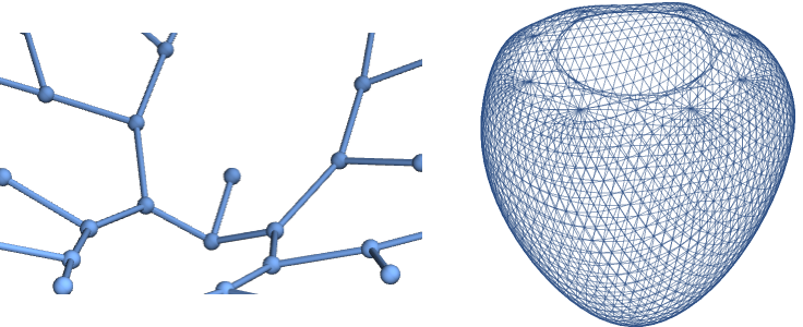
GraphPlot3D[SimpleGraph[Table[iMod[i ^ 2, 75], {i, 75}]], EdgeShapeFunction -> ({Cylinder[#1, 0.1]}&), VertexShapeFunction -> ({Sphere[#, 0.3]}&)]Structure an engineering matrix:
GraphPlot3D[ExampleData[{"Matrix", "HB/dwt_1005"}, "Matrix"], VertexShapeFunction -> None]Properties & Relations (7)
Use LayeredGraphPlot for hierarchical-style drawing of directed graphs:
LayeredGraphPlot[{{"main" -> "fun1", "fun1[a,b]"}, {"main" -> "fun2", "fun2[1,2,3]"}, {"fun2" -> "fun3", "fun3[0.5]"}, {"main" -> "fun3", "fun3[0.6]"}}, PlotTheme -> "DiagramBlue"]Use TreePlot for different types of tree drawing:
TreePlot[Flatten[Table[{i -> 2i + j - 1}, {j, 2}, {i, 7}]]]Use GraphPlot to draw graphs in 2D:
GraphPlot[Table[i -> Mod[i ^ 2, 200], {i, 200}]]Use GraphData for an extensive collection of predefined graphs and properties:
Short[GraphData[], 3]Get the connectivity and plot it:
GraphData["DesarguesGraph", "EdgeRules"]GraphPlot3D[%]Use PolyhedronData for a large collection of polyhedra and properties:
PolyhedronData["Dodecahedron", "Skeleton", "Rule"]GraphPlot3D[%]Compare to a predefined embedding:
PolyhedronData["Dodecahedron", "Skeleton"]Use ExampleData for a large collection of sparse matrices:
GraphPlot3D[ExampleData[{"Matrix", "HB/can_229"}, "Matrix"]]Use ArrayPlot or MatrixPlot to display sparse matrices:
g = ExampleData[{"Matrix", "Bai/bfwa62"}, "Matrix"]{ArrayPlot[g], MatrixPlot[g]}Text
Wolfram Research (2007), GraphPlot3D, Wolfram Language function, https://reference.wolfram.com/language/ref/GraphPlot3D.html (updated 2019).
CMS
Wolfram Language. 2007. "GraphPlot3D." Wolfram Language & System Documentation Center. Wolfram Research. Last Modified 2019. https://reference.wolfram.com/language/ref/GraphPlot3D.html.
APA
Wolfram Language. (2007). GraphPlot3D. Wolfram Language & System Documentation Center. Retrieved from https://reference.wolfram.com/language/ref/GraphPlot3D.html