

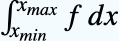





Integrate


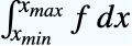

詳細とオプション
- Integrate[f,x]は ∫fx として入力できる.
- ∫ は,
 int
 または\[Integral]として入力できる.
- は通常のdと異なり,
 dd
 または\[DifferentialD]として入力される.
- Integrate[f,{x,y,…}∈reg]は ∫{x,y,…}∈regf として入力できる.
- Integrate[f,{x,xmin,xmax}]は,xminを ∫の下付き文字として,xmaxを上付き文字として表すことによって入力できる.
- 多重積分は,標準的な反復表記の変形を使用する.第1変数は,最も外側の積分に対応して与えられ,これが最後に実行される. »
- Integrateは,有理関数の積分を評価することができる.また,結果が同じ関数の組で表すことができる範囲で指数関数,対数関数,三角関数,そして逆三角関数の積分を評価することができる.
- Integrateは,多くの特別関数によって結果を与えることができる.
- Integrateは,明示的に積分できないものについてはある種の簡約化を実行する.
- 定積分については,Nを適用することで数値的な結果を得ることができる. »
- 新しいクラスの積分に結果を与えるために,Integrateが関わるパターンに値を割り当てることができる.
- 積分変数は x[i]のような構造や,頭部が数学関数ではない任意の式でもよい.
- 不定積分において,Integrateは,ほとんどすべてのパラメータの値に対して正しい結果を求める.
- 定積分において指定可能なオプション
-
Assumptions $Assumptions パラメータについての仮定を指定 GenerateConditions Automatic パラメータについての制約条件を含む解を生成するかどうか GeneratedParameters None 生成されたパラメータにどのように名前を付けるか PrincipalValue False コーシー主値を求めるかどうか - Integrateは,標準的な公式集に載っているすべての不定積分とほとんどの定積分が評価できる.
- StandardFormでは,Integrate[f,x]は ∫fx として出力される.
例題
すべて開く すべて閉じる例 (4)
Integrate[x ^ 2 + Sin[x], x]Integrate[1 / (x ^ 3 + 1), {x, 0, 1}]Plot[(1/x^3 + 1), {x, 0, 1}, Filling -> Axis]
 を使って

 使って
∫Sqrt[x + Sqrt[x]]ⅆxTraditionalForm[%] を使って下限を,
 を使って上限を入力する:
Subsuperscript[∫, 0, ∞]Log[x] Exp[-x^2]ⅆxスコープ (78)
基本的な用法 (13)
int = Integrate[1 / (x ^ 3 + 1), x]D[int, x]//Simplify intt
 を使ってテンプレート
 を入力し,
 を使ってフィールド間を移動する:
∫(a x ^ 2 + b x + c)ⅆxIntegrate[x ^ 2, x, GeneratedParameters -> C]Integrate[(2x + 3) / (x ^ 2 + 5x + 6), {x, 0, 2}]Integrate[BesselJ[2, x] / (1 + x ^ 2), {x, 0, ∞}]Integrate[Sin[x] / x, {x, -∞, ∞}] dintt
 を使ってテンプレート
 を入力し,
 を使ってフィールド間を移動する:
Subsuperscript[∫, 0, π]Cos[x]ⅆxIntegrate[(a x/x^3 + 2), {x, 1, ∞}]Integrate[Exp[-c x^2], {x, -∞, ∞}]Integrate[Exp[-c x^2], {x, -∞, ∞}, Assumptions -> Re[c] == 0]Integrate[(BesselJ[3, y]/x + 1), {x, 0, 5}, {y, 0, 5}]Integrate[Exp[-x + y], {x, 0, ∞}, {y, 0, 1}]Integrate[Sin[x y], {x, 0, 1}, {y, 0, x}]StandardFormでは,y が x の前に置かれる:
Subsuperscript[∫, 0, 1]Subsuperscript[∫, 0, x]Sin[x y]ⅆyⅆxPlot3D[Sin[x y], {x, y}∈Triangle[{{0, 0}, {0, 1}, {1, 0}}]]Integrate[1, {x, y}∈Circle[]]記号 ∈ は  el
 または ∈ と入力する:
Integrate[1, x∈Ball[3]] を使って下付き文字として領域指定
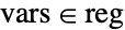
Underscript[∫, {x, y, z}∈Tetrahedron[]](x^4 y^5 + z^10) rintt
 を使ってテンプレート
 を入力し,
 を使ってフィールド間を移動する:
Underscript[∫, {x, y}∈Rectangle[]]x y^2Integrate[f'[x], x]Integrate[((1 - f[x])f'[x]) / E ^ f[x], x]Integrate[{x, (1/Sqrt[x]), Sin[x]}, {x, 0, 5}]Integrate[(| | | |
| ------- | ------- | ------- |
| x | Sqrt[x] | x^1 / 3 |
| Sqrt[x] | x^1 / 3 | x^1 / 4 |
| x^1 / 3 | x^1 / 4 | x^1 / 5 |), {x, 0, 5}]//MatrixForm記号積分に失敗すると,NIntegrateが自動的に呼び出される:
Integrate[E ^ (-x ^ x), {x, 0, 1}]N[%]不定積分 (10)
∫x^nⅆx∫(1/x)ⅆx∫Sin[x]ⅆx∫Exp[x]ⅆxIntegrate[Exp[x], x, GeneratedParameters -> C]∫Sec[x]^2ⅆx∫Cot[x]ⅆx∫Sec[x]ⅆxD[%, x]//Simplifyflist = {x ^ n, 1 / x, b^x, Log[x], Sin[x], Cos[x], (1/x^2 + a^2), (1/x^2 - a^2)};Grid[Prepend[Transpose[{flist, Integrate[flist, x]}], {f[x], ∫f[x]ⅆx}], IconizedObject[«Grid options»]]//TraditionalFormIntegrate[1 / (x ^ 4 - 1), x]Integrate[( x + 1/a^2 x^2 + c^2), x]これらはRootオブジェクトの和を含むことがある:
Integrate[1 / (x ^ 5 + 2x + 1), x]∫ArcSin[x]ⅆx∫Cosh[x]ⅆx∫(x^2/Sqrt[a^2 + x^2])ⅆx∫Exp[a x]Cos[b x]ⅆxIntegrateは,該当する場合は,複素平面上で有効な不定積分を返す:
intℂ[x_] = ∫Tan[x]ⅆxD[intℂ[x], x]

intℝ[x_] = Log[RealAbs[Sec[x]]];
Simplify[D[intℝ[x], x]]FullSimplify[Re[intℂ[x]] == Re[intℝ[x]]]Plot[{Re[intℂ[x]], Re[intℝ[x]]}, {x, 0, 4Pi}, PlotTheme -> {"Detailed", "NeonColors", "DashedLines"}]

Plot[{Im[intℂ[x]], Im[intℝ[x]], Cos[x]}, {x, 0, 4Pi}, PlotTheme -> {"Detailed", "NeonColors", "DashedLines"}]Integrate[Sqrt[x]Sqrt[1 + x], x]Integrate[Sqrt[x]Sqrt[1 + x]Sqrt[2 + x], x]Erfのような特殊関数についてのみ実行できる積分が多数ある:
Integrate[Exp[-x ^ 2], x]PolyLogやLogIntegralのようなLogの一般化:
Integrate[Log[1 + x] ^ 2 / x, x]Integrate[Log[Log[x]], x]Hypergeometric2F1のような超幾何関数:
Integrate[Tan[x] ^ n, x]flist = {BesselJ[0, x], Erf[x], EllipticE[x], Sqrt[x]PolyLog[2, x], AiryAi[x], SinhIntegral[2 / (x + 1)]};Grid[Prepend[Transpose[{flist, Integrate[flist, x]}], {f[x], ∫f[x]ⅆx}], IconizedObject[«Grid options»]]//TraditionalFormIntegrate[p[x]Log[p[x]], p[x]]定積分 (13)
Integrate[x ^ 4 + x ^ 2 + 1, {x, 1, 3}]Plot[x ^ 4 + x ^ 2 + 1, {x, 1, 3}, Filling -> Axis]Integrate[a x ^ 2 + b x + c, {x, -2, 2}]Integrate[x ^ n + n x, {x, 0, a}, Assumptions -> n > 1 && n∈ℤ]Integrate[1 / (x ^ 4 + x ^ 2 + 1), {x, 0, Infinity}]Plot[(1/x^4 + x^2 + 1), {x, 0, 5}, Filling -> Axis, PlotRange -> All, Epilog -> {RGBColor[0.368417, 0.506779, 0.709798], Arrow[{{0, 0}, {5, 0}}]}]Integrate[(4x ^ 2 - 7x - 12) / ((x + 2)(x - 3)), {x, -1, 2}]Plot[(4 x^2 - 7 x - 12/(x + 2) (x - 3)), {x, -1, 2}, Filling -> 0, PlotRange -> All]Integrate[(1 + x^3) CubeRoot[x], {x, -1, 1}]Plot[(1 + x^3) CubeRoot[x], {x, -1, 1}, Filling -> Axis, FillingStyle -> {RGBColor[0.95, 0.627, 0.1425, 0.2], RGBColor[0.24, 0.6, 0.8, 0.2]}]Integrate[1 / ((2 + x ^ 2)Sqrt[4 + 3x ^ 2]), {x, -∞, ∞}]Plot[(1/(2 + x^2) Sqrt[4 + 3 x^2]), {x, -7, 7}, Filling -> 0, AxesOrigin -> {0, 0}, Epilog -> {RGBColor[0.368417, 0.506779, 0.709798], Arrowheads[{-Medium, Medium}], Arrow[{{-7, 0}, {7, 0}}]}]Integrate[Cos[2x] ^ 4, {x, 0, π}]Plot[Cos[2x] ^ 4, {x, 0, π / 2}, Filling -> Axis]Integrate[x ^ 2Sin[2x], {x, 0, 2π}]Plot[x ^ 2Sin[2x], {x, 0, 2π}, Filling -> Axis, FillingStyle -> {RGBColor[0.95, 0.627, 0.1425, 0.2], RGBColor[0.24, 0.6, 0.8, 0.2]}]Integrate[x ^ 5Log[x], {x, 1, 2}]Plot[x ^ 5Log[x], {x, 1, 2}, Filling -> Axis]Integrate[Exp[-x + Exp[-x]], {x, 0, ∞}]Plot[Exp[-x + Exp[-x]], {x, 0, 4}, PlotRange -> Full, Filling -> Axis, Epilog -> {RGBColor[0.368417, 0.506779, 0.709798], Arrowheads[Medium], Arrow[{{0, 0}, {4, 0}}]}]Integrate[x Cosh[x], {x, 0, a}]Integrate[x^2 Sech[x]^2, {x, -∞, ∞}]Integrate[x / Sqrt[1 - x], {x, 0, 1}]Plot[x / Sqrt[1 - x], {x, 0, 1}, Filling -> Axis]これは,より小さい区間上の積分の結果の極限として見ることができる:
Underscript[, a -> 1^ - ]Subsuperscript[∫, 0, a](x/Sqrt[1 - x])ⅆxarea = Subsuperscript[∫, -1, 1](x^2/Sqrt[1 - x^4])ⅆx%//NPlot[(x^2/Sqrt[1 - x^4]), {x, -1, 1}, Filling -> 0]これは,より小さい区間上の積分の結果の多変量極限として見ることができる:
area == Limit[Integrate[(x^2/Sqrt[1 - x^4]), {x, a, b}, Assumptions -> -1 < a < b < 1], {a, b} -> {-1, 1}, Direction -> {"FromAbove", "FromBelow"}]無限区間上での積分は有限領域上の積分の極限と見ることができる:
Integrate[x E ^ (-x), {x, 1, ∞}]


% == Underscript[, a -> ∞]Integrate[x E ^ (-x), {x, 1, a}]Subsuperscript[∫, -∞, ∞]E^-x^2ⅆx% == Underscript[, {a, b} -> {-∞, ∞}]Subsuperscript[∫, a, b]E^-x^2ⅆxパラメータがある場合は,収束を確かなものとする条件が報告されるかもしれない:
Integrate[x ^ n, {x, 0, 1}]Integrate[E ^ (a x), {x, 0, ∞}]Integrate[Sin[t] / t, {t, a, b}]Integrate[Cos[Sin[x] ^ 2], {x, 0, 2π}]%//NPlot[Cos[Sin[x] ^ 2], {x, 0, 2π}, Filling -> 0, PlotRange -> {0, 1}]flist = {BesselJ[2, x] / x, BesselK[0, x] ^ 2, AiryAi[x] ^ 2, Exp[-x] Sinc[x], Sin[x]Erfc[x]};Grid[Prepend[Transpose[{flist, Subsuperscript[∫, 0, ∞]flistⅆx}], {f[x], Subsuperscript[∫, 0, ∞]f[x]ⅆx}], IconizedObject[«Grid options»]]//TraditionalFormIntegrate[Sqrt[x], {x, I, 3 - I}]Integrate[(1/z + 1 / 2), {z, 1, E^(I π/3), E^(2 I π/3), -1, E^-(2 I π/3), E^-(I π/3), 1}]//FullSimplifyIntegrate[(I Exp[I ω]/Exp[I ω] + 1 / 2), {ω, 0, 2π}]ComplexPlot[(1/z + 1 / 2), {z, -1.2 - 1.2I, 1.2 + 1.2I}, Epilog -> {Thick, Arrowheads[Medium], White, Arrow[{{1, -.05}, {1, 0}}], Circle[], Dashed, Black, Arrow[ReIm /@ Exp[2π I / 6 Range[0, 6]]]}]区分関数と一般化された関数の積分 (12)
Piecewise関数の不定積分を計算する:
f[x_] := Piecewise[{{-x^2, x < 0}, {x^2, True}}]∫f[x]ⅆxSimplify[D[%, x] == f[x]]不連続Piecewise関数を積分する:
f[x_] := Piecewise[{{-x + 1, x < 0}, {x, 0 < x < 1}, {x^2, True}}]g[x_] = ∫f[x]ⅆxResolve[ForAll[x, x != 0 && x∈ℝ, Derivative[1][g][x] == f[x]]]Plot[{f[x], g[x]}, {x, -2, 2}, PlotTheme -> {"Detailed", "DashedLines"}]unitInt[x_] = Integrate[x UnitStep[x], x]Plot[{x UnitStep[x], unitInt[x]}, {x, -2, 2}, PlotTheme -> {"Detailed", "DashedLines"}]clipInt[x_] = Integrate[Clip[x] ^ 2, x]Plot[{Clip[x] ^ 2, clipInt[x]}, {x, -2, 2}, PlotTheme -> {"Detailed", "DashedLines"}]maxInt[x_] = Integrate[Max[Sin[x], Cos[x]], x]定義されているすべての場所で,maxIntの導関数はもとの関数と等しくなる:
Simplify[D[maxInt[x], x] == Max[Sin[x], Cos[x]]]Plot[{Max[Sin[x], Cos[x]], maxInt[x]}, {x, 0, 4Pi}, PlotTheme -> {"Detailed", "DashedLines"}]Piecewise関数の定積分を計算する:
f[x_] := Piecewise[{{1, x < 2}, {x^3, 2 < x < 3}}, 0]Integrate[f[x], {x, 0, 3}]int[x_] = Integrate[f[t], {t, 0, x}, Assumptions -> x > 0]Plot[{f[x], int[x]}, {x, 0, 4}, PlotTheme -> {"Detailed", "DashedLines"}]Floorのような区分関数の定積分を計算する:
Integrate[Floor[x ^ 2], {x, 0, 3}]Plot[Floor[x ^ 2], {x, 0, 3}, Filling -> Axis]Integrate[PrimePi[n], {n, 0, 100}]Plot[PrimePi[x], {x, 0, 100}, Filling -> Axis]Integrate[Ceiling[x ^ 2 + TriangleWave[x]], {x, -2, 2} ]f[x_] := x ^ 2 UnitStep[x + 1]int[a_] = Integrate[f[x], {x, -3, a}]Plot[{f[a], int[a]}, {a, -2, 2}, PlotTheme -> {"Detailed", "DashedLines"}]f[x_] := Max[Sin[x], Cos[x]]f[x]//PiecewiseExpandAssumptionsを使って有限数の場合で積分する:
maxInt[a_] = Integrate[f[x], {x, 0, a}, Assumptions -> 0 < a < 2Pi]Plot[{f[a], maxInt[a]}, {a, 0, 2Pi}, PlotTheme -> {"Detailed", "DashedLines"}]Integrate[DiracDelta[x], {x, -∞, ∞}]Integrate[Sin[x] ^ 2 HeavisideTheta[x + π]HeavisideTheta[π - x], {x, -∞, ∞}]Integrate[DiracDelta[Cos[x ^ 2 - 1]], {x, -2, 2}]Integrate[DiracDelta[x], x]Integrate[DiracDelta[x], x, x]Integrate[f[x] DiracDelta[x - a], {x, -1, 1}, Assumptions -> a∈Reals]Integrate[Cos[x - a] HeavisideLambda[x], {x, 0, Pi}, Assumptions -> a∈Reals]f = Interpolation[{10, -5, 10, -10, 20}]g = Head[Integrate[f[x], x]]g'[3.5] == f[3.5]Plot[{f[x], g[x]}, {x, 1, 5}, PlotTheme -> {"Detailed", "DashedLines"}]ネストした積分 (12)
Integrate[a x ^ 2 + b x + c, x, x]//ExpandD[%, {x, 2}]∫∫∫(1/x^2 + 4)ⅆxⅆxⅆxFullSimplify[D[%, {x, 3}]]Integrate[x ^ 2Sin[y], y, x]D[%, x, y]Integrate[x, x, GeneratedParameters -> C]Integrate[x, x, x, GeneratedParameters -> C]D[%, x, x]2つの変数についてのネストした積分についての2つの積分関数を生成する:
Integrate[x, x, y, GeneratedParameters -> C]D[%, x, y]

Integrate[Exp[x]Cos[y], {x, 0, a}, {y, 0, b}]Subsuperscript[∫, 0, a]Subsuperscript[∫, 0, b]Exp[x]Cos[y]ⅆyⅆxSubsuperscript[∫, 0, b]Subsuperscript[∫, 0, a]Exp[x]Cos[y]ⅆxⅆyIntegrate[(x + y), {y, 0, 1}, x]Integrate[x ^ 2y / (x + y), {x, 0, 3}, {y, 1, 2}]Plot3D[(x^2 y/x + y), {x, 0, 3}, {y, 1, 2}, Filling -> Axis, FillingStyle -> Opacity[0.6], Mesh -> None]Integrate[y Sin[x y], {x, 1, 4}, {y, 0, π}]負の体積(薄い青)と正の体積(濃い灰色)が同じくらいである:
Plot3D[{y Sin[x y], 0}, {x, 1, 4}, {y, 0, π}, IconizedObject[«Plot3D options»]]Subsuperscript[∫, -2, 2]Subsuperscript[∫, 2 x^2, 4 + x^2](8 - (3 y/3) - (3 x y/3) + (x^2 y/3) + (x^3 y/3))ⅆyⅆxPlot[{2x ^ 2, 4 + x ^ 2}, {x, -2, 2}, Filling -> {1 -> {2}}, PlotLegends -> "Expressions"]Plot3D[8 - (3 y/3) - (3 x y/3) + (x^2 y/3) + (x^3 y/3), {x, y}∈ImplicitRegion[-2 < x < 2 && 2 x^2 < y < 4 + x^2, {x, y}], FillingStyle -> Opacity[.5], Filling -> Axis, PlotRange -> All, ViewPoint -> {.3, 3.1, 1.3}, Mesh -> None]Integrate[Cos[z]Exp[x]y, {x, 0, 1}, {y, -1, 2}, {z, 0, 3}]RegionPlot3D[0 < x < 1 && -1 < y < 2 && 0 < z < 3, {x, -0.5, 1.5}, {y, -1.5, 2.5}, {z, -0.5, 3.5}]Integrate[Sqrt[x ^ 2 + z ^ 2]y, {x, -2, 2}, {y, x ^ 2, 4}, {z, -Sqrt[y - x ^ 2], Sqrt[y - x ^ 2]}]//FullSimplifyRegionPlot3D[y > x ^ 2 + z ^ 2 && 0 < y < 4, {x, -3, 3}, {y, -0.5, 4.5}, {z, -3, 3}]Integrate[a b ^ 2 - c / d ^ e, {a, 0, 1}, {b, 1, 2}, {c, 2, 3}, {d, 3, 4}, {e, 4, 5}]N[%]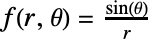
f[r_, θ_] := (Sin[θ]/r)CoordinateChartDataで超球面座標の座標範囲を見る:
CoordinateChartData["Hyperspherical", "CoordinateRangeAssumptions", {r, θ, φ, ψ}]CoordinateChartData["Hyperspherical", "VolumeFactor", {r, θ, φ, ψ}]Subsuperscript[∫, -π, π]Subsuperscript[∫, 0, π]Subsuperscript[∫, 0, π]Subsuperscript[∫, 0, R]f[r, θ](r^3 Sin[θ]^2 Sin[φ])ⅆrⅆθⅆφⅆψ領域積分 (11)
Integrate[1, {x, y}∈Disk[]]Underscript[∫, {x, y}∈Disk[]]1同様に,Booleを使って長方形領域上で円板に限定して積分する:
Integrate[Boole[x ^ 2 + y ^ 2 ≤ 1], {x, -1, 1}, {y, -1, 1}]Subscript[∫, {x, y}∈Disk[]](Cos[3x]Sin[5y] + x^2)Booleを使って表現された同じ積分:
Subsuperscript[∫, -1, 1]Subsuperscript[∫, -1, 1](Cos[3x]Sin[5y] + x^2)Boole[x^2 + y^2 ≤ 1]ⅆyⅆxSubsuperscript[∫, -1, 1]Subsuperscript[∫, -Sqrt[1 - x^2], Sqrt[1 - x^2]](Cos[3x]Sin[5y] + x^2)ⅆyⅆxPlot3D[Cos[3x]^2Sin[5y] + 1, {x, y}∈Disk[], Filling -> 0, Mesh -> None, FillingStyle -> Automatic]Integrate[Sin[b x], {x}∈Interval[{0, Pi}]]Integrate[Sin[b x], {x, 0, Pi}]GenerateConditions Trueのとき,領域が退化しないように仮定が生成される:
Integrate[x^2y, {x, y}∈Rectangle[{0, 0}, {a, b}], GenerateConditions -> True]Integrate[x^2y, {x, 0, a}, {y, 0, b}, GenerateConditions -> True]Subscript[∫, {x, y}∈Circle[]](x^2 y + y^2/2)Subsuperscript[∫, -Pi, Pi](Cos[θ]^2Sin[θ] + Sin[θ]^2/2)ⅆθ
Underscript[∫, {x, y, z}∈Sphere[{x0, y0, z0}, r]](1/(x - x0)^2 + (y - y0)^2 + (z - z0)^2)Integrate[1, {x, y, z}∈Point[{{1, 2, 3}, {4, 5, 6}, {7, 8, 9}}]]int1 = Integrate[Boole[1 < x ^ 2 - y ^ 2 < 4 && x y < 1 && x > 0 && y > 0], {x, -∞, ∞}, {y, -∞, ∞} ]ImplicitRegionとして領域を定義し,この領域上で直接積分する:
reg = ImplicitRegion[1 < x ^ 2 - y ^ 2 < 4 && x y < 1 && x > 0 && y > 0, {x, y}];int2 = Integrate[1, {x, y}∈reg]FullSimplify[int1 - int2]RegionPlot[reg]reg = ImplicitRegion[x + 2y + 3z < 2 && -1 < x < y < z < 1, {x, y, z}];Subscript[∫, {x, y, z}∈reg](x^2 + 2y z)RegionPlot3Dを使って3D領域を可視化する:
RegionPlot3D[reg, PlotPoints -> 65, PlotTheme -> "FrameGrid"]Integrate[ (x ^ 2 + y ^ 2) Boole[0 ≤ z ≤ 1 && x ^ 2 + y ^ 2 ≤ z ^ 2], {x, -∞, ∞}, {y, -∞, ∞}, {z, -∞, ∞} ]RegionPlot3D[0 ≤ z ≤ 1 && x ^ 2 + y ^ 2 ≤ z ^ 2, {x, -1, 1}, {y, -1, 1}, {z, 0, 1}]Integrate[Boole[ax < y], {x, 0, 1}, {y, 0, 1}]reg = ImplicitRegion[Sin[x] > 1 / 2, {{x, 0, ∞}}];Underscript[∫, {x}∈reg]Exp[-x]積分の記号的な特徴 (7)
Integrate[f''[x] + 2 a f'[x], x]Integrate[f[t], {t, 0, x}]D[%, x]Subscript[∂, x]Subsuperscript[∫, a[x], b[x]]f[t]ⅆtIntegrate[f[x, a], {x, 0, 1}]D[%, a]Subscript[∂, a]Subsuperscript[∫, p[a], q[a]]f[x, a]ⅆxInactive[Integrate][1 / (1 + x), x]D[%, x]Inactivate[∫x^nⅆx, Integrate] == ∫x^nⅆxInactivate[∫(1/Sqrt[1 - x^2])ⅆx, Integrate] == ∫(1/Sqrt[1 - x^2])ⅆxActivate[{Inactive[Integrate][x^n, x] == (x^1 + n/1 + n), Inactive[Integrate][1/Sqrt[1 - x^2], x] == ArcSin[x]}]Inactivate[Integrate[D[f[x, a], a], x] == ((D[Integrate[f[x, a], x], a]))]Activate[Inactive[Integrate][Inactive[D][Inactive[f][x, a], a], x] == Inactive[D][Inactive[Integrate][Inactive[f][x, a], x], a]]積分のLaplaceTransformを計算する:
LaplaceTransform[Integrate[f[u], {u, 0, t}], t, s]オプション (11)
Assumptions (3)
デフォルトで,収束を確かなものとするパラメータについての条件が生成される:
Integrate[x ^ n, {x, 0, 1}]Assumptionsを使うと,与えられた仮定の下で有効な結果が返される:
Integrate[x ^ n, {x, 0, 1}, Assumptions -> n > 0]Assumptionsを手動で指定して,自動的に生成された条件外の値を確かめる:
Integrate[Exp[-a x^2], {x, -∞, ∞}]
Integrate[Exp[-a x^2], {x, -∞, ∞}, Assumptions -> Re[a] == 0]Integrate[Floor[x], x]Integrate[Floor[x], x, Assumptions -> 0 < x < 5]GenerateConditions (2)
デフォルトで,一変量の定積分は収束を確かなものとするパラメータについて条件を生成する:
Integrate[Exp[-a x ^ 2], {x, 0, ∞}]Integrate[Exp[-a x ^ 2], {x, 0, ∞}, GenerateConditions -> False]GenerateConditions->Falseを使って積分速度を上げる:
Integrate[x ^ n, {x, -1, b}, GenerateConditions -> False]//TimingIntegrate[ x ^ n, {x, -1, b}, GenerateConditions -> True]//TimingGeneratedParameters (4)
Integrate[x, x]GeneratedParametersの値を指定して一般的な不定積分を得る:
Integrate[x, x, GeneratedParameters -> C]Integrate[Exp[2x], x, x, GeneratedParameters -> C]Integrate[Exp[2x], x, x, x, GeneratedParameters -> C]入力式にすでに生成されたパラメータが含まれている場合は,使用可能な次の指標が使われる:
Integrate[(E^2 x/8) + C[3], x, GeneratedParameters -> C]複数の変数を持つネストした積分の場合は,不定積分が任意の関数を含む:
Integrate[Exp[2x], x, y, GeneratedParameters -> C]Integrate[Exp[2x], x, y, z, GeneratedParameters -> C]D[%, x, y, z]GeneratedParametersの値が生成された各パラメータの指標に適用される:
Integrate[Cos[x], x, x, GeneratedParameters -> f]Integrate[Cos[x], x, x, GeneratedParameters -> (Subscript["const", #]&)]Noneという値は生成されたパラメータを無効にする:
Integrate[Cos[x], x, x, GeneratedParameters -> None]PrincipalValue (2)
Integrate[1 / x, {x, -1, 2}]
Integrate[1 / x, {x, -1, 2}, PrincipalValue -> True]Underscript[, a -> 0^ + ](Subsuperscript[∫, -1, -a](1/x)ⅆx + Subsuperscript[∫, a, 2](1/x)ⅆx)Integrate[Tan[x], {x, 0, π}]

Integrate[Tan[x], {x, 0, π}, PrincipalValue -> True]Plot[Tan[x], {x, 0, Pi}, Filling -> Axis, FillingStyle -> {RGBColor[0.95, 0.627, 0.1425, 0.2], RGBColor[0.24, 0.6, 0.8, 0.2]}]アプリケーション (67)
積分の幾何学 (5)
定数関数  の積分
 は,高さ
 ,幅
 の長方形の符号付き面積である:
Subsuperscript[∫, 1, 4]2ⅆx% == 2×(4 - 1)Subsuperscript[∫, 1, 4](-1)ⅆx% == (-1)×(4 - 1)Plot[{2, -1}, {x, 1, 4}, Filling -> Axis]区分定数関数の積分 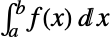 はそのプロットで定義される長方形の符号付き面積の和である:
f[x_] := Piecewise[{{0, x < 0}, {1, Inequality[0, LessEqual, x, Less, 1]},
{-2, Inequality[1, LessEqual, x, Less, 3]}, {5, 3 <= x}}]Subsuperscript[∫, 0, 4]f[x]ⅆx% == 1×(1 - 0) + (-2)(3 - 1) + 5×(4 - 3)Plot[f[x], {x, 0, 4}, Filling -> Axis, FillingStyle -> {RGBColor[0.95, 0.627, 0.1425, 0.2], RGBColor[0.24, 0.6, 0.8, 0.2]}]一般的な関数の積分 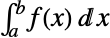 は,そのプロットと水平軸の間の符号付き面積である:
f[x_] := x ^ 2 + 1Integrate[f[x], {x, 0, 2}]Plot[f[x], {x, 0, 2}, Filling -> Axis, AxesOrigin -> {0, 0}]これは,そのプロットで定義された長方形について考えると,区分定数の場合と関連している:
rectangles[f_, a_, b_, n_] := {Opacity[0.75], StandardOrange, N@Table[Rectangle[{a + k(b - a) / n, 0}, {a + (k + 1)(b - a) / n, f[a + k(b - a) / n]}], {k, 0, n - 1}]}区間[0,2]上の n5についての長方形は以下のようになる:
Plot[f[x], {x, 0, 2}, Epilog -> rectangles[f, 0, 2, 5], AxesOrigin -> {0, 0}]これらの長方形の面積は,曲線の下の面積を近似するリーマン和を定義する:
RiemannSum[f_, a_, b_, n_] :=
Sum[f[(a + (b - a)k / n)], {k, 0, n - 1}] (b - a) / nRiemannSum[f, 0, 2, n]DiscreteLimitを使って,Integrateと同じように, のときに厳密な答を得る:
DiscreteLimit[%, n -> ∞]label[f_, a_, b_, n_] := StringForm["TraditionalFormSubscriptBox[A, curve] == ``\ \ \ SubscriptBox[A, rects] = ``", NumberForm[N@Subsuperscript[∫, a, b]f[x]ⅆx, {4, 3}], NumberForm[N@RiemannSum[f, a, b, n], {4, 3}]]With[{a = 0, b = 2}, Manipulate[Plot[fn[x], {x, a, b}, Filling -> Axis, AxesOrigin -> {0, 0}, Epilog -> rectangles[fn, a, b, 2^n], PlotLabel -> label[fn, a, b, 2^n]], {{n, 1, Dynamic@StringForm["n = ``", 2^n]}, 1, 12, 1}, {{fn, f}, {f, CubeRoot, Sin, Abs[2# - 1]& -> HoldForm@2x - 1}}, SaveDefinitions -> True]]微積分の基本定理は,関数を固定下限から可変上限までの積分に関連付ける:
f[x_] := Sqrt[x ^ 2 + 1]

g[x_] = Integrate[f[t], {t, 0, x}, Assumptions -> x > 0]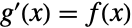
Simplify[g'[x] == f[x]]Limit[(g[x + h] - g[x]/h), h -> 0] は,
 についての次の表で説明されているように,高さ
 で幅
 の長方形と
 で消えてしまう小さい修正からなる面積であることに注意のこと:
TableForm[Table[{h, (g[1 + h] - g[1]/h), (g[1 + h] - g[1]/h) - f[1]}, {h, {.1, .05, .001, 0.0005, 0.00001, 0.00000005}}], TableHeadings -> {{}, {h, HoldForm[(g[1 + h] - g[1]/h)], HoldForm[(g[1 + h] - g[1] - f[1]h/h)]}}]したがって,極限は,次の可視化で説明されるように,幾何学的に  に等しいものと見ることができる:
title[u_, k_] := IconizedObject[«Code for plot title»]labels[u_, k_] := IconizedObject[«Code for labels in plot»]Manipulate[Plot[{Piecewise[{{f[s], 0 ≤ s ≤ u}, {Undefined, True}}], Piecewise[{{f[s], u ≤ s ≤ u + k}, {Undefined, True}}], f[s]}, {s, 0, 3}, PlotLabel -> title[u, k], Epilog -> labels[u, k], IconizedObject[«More Plot options»]], {{u, 1.5, Style[x, Italic, 14]}, 1, 2, Appearance -> {"Labeled"}, LabelStyle -> 14}, {{k, .25, Style[h, Italic, 14]}, 0.00001, .5, Appearance -> "Labeled", LabelStyle -> 14}, SaveDefinitions -> True]Interpolationでデータの離散集合を積分する:
data = Table[{x, Sin[(1/x + 1 / 2)]}, {x, 0, 10, 0.25}];Integrate[Interpolation[data][x], {x, 0, 10}]Integrate[Sin[(1/x + 1 / 2)], {x, 0, 10}]//N{ListLinePlot[data, Filling -> Axis, ImageSize -> Small, InterpolationOrder -> 0], Plot[Interpolation[data][x], {x, 0, 10}, Filling -> Axis, ImageSize -> Small]}曲線間の面積 (7)



Plot[1 + Sqrt[9 - x ^ 2], {x, -3, 0}, Filling -> Axis, AxesOrigin -> {0, 0}]Integrate[1 + Sqrt[9 - x ^ 2], {x, -3, 0}]


Plot[Sin[x] ^ 2 Cos[x] ^ 4, {x, -π, π}, Filling -> Axis]Integrate[Sin[x] ^ 2 Cos[x] ^ 4, {x, -π, π}]

Plot[Sin[x], {x, -π, π}, Filling -> Axis]Integrate[RealAbs[Sin[x]], {x, -π, π}]同様に,これを上下の間の差の2つの積分の和として計算することもできる:
Subsuperscript[∫, -π, 0](0 - Sin[x])ⅆx + Subsuperscript[∫, 0, π](Sin[x] - 0)ⅆx


Plot[{5x - x ^ 2, x}, {x, 0, 4}, PlotLegends -> "Expressions", Filling -> {1 -> {2}}]Integrate[(5x - x ^ 2) - (x), {x, 0, 4}]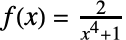
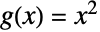
pts = Solve[y == 2 / (1 + x ^ 4) && y == x ^ 2, {x, y}, Reals]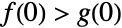


Integrate[2 / (x ^ 4 + 1) - x ^ 2, {x, -1, 1}]%//NShow[RegionPlot[x^2 < y < (2/x^4 + 1), {x, -1, 1}, {y, 0, 2}], Plot[{2 / (1 + x ^ 4), x ^ 2}, {x, -2, 2}, PlotLegends -> "Expressions"], PlotRange -> All]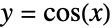
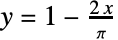
pts = Solve[y == Cos[x] && y == 1 - 2x / π && 0 ≤ x ≤ π, {x, y}]Integrate[RealAbs[Cos[x] - (1 - 2x / π)], {x, 0, π}]//ExpandShow[RegionPlot[y ≤ Cos[x] && y ≥ 1 - 2x / π || y ≥ Cos[x] && y ≤ 1 - 2x / π, {x, 0, π}, {y, -2, 2}, PlotPoints -> 60, PlotStyle -> Opacity[.75]], Plot[{Cos[x], 1 - 2x / π}, {x, -1, 4}, PlotTheme -> "Detailed"], Graphics[{PointSize[Large], Point[{x, y} /. pts]}], PlotRange -> All, Axes -> True]プロットを使って絶対値なしで積分を等しい2つの積分に分割する:
Subsuperscript[∫, 0, (π/2)](Cos[x] - (1 - (2 x/π)))ⅆx + Subsuperscript[∫, (π/2), π]((1 - (2 x/π)) - Cos[x])ⅆx ,
 ,
 で囲まれた部分の面積を計算するために,まず交差する点を求める:
pt1 = Solve[y == 1 / x ^ 2 && y == x, {x, y}, Reals]pt2 = Solve[y == 1 / x ^ 2 && y == (1 / 8)x, {x, y}, Reals]pt3 = Solve[y == (1 / 8)x && y == x, {x, y}, Reals]ContourPlot[{y == 1 / x ^ 2, y == x, y == (1 / 8)x}, {x, -1, 3}, {y, -1, 2}, PlotLegends -> "Expressions", Axes -> True, AspectRatio -> Automatic, Epilog -> {PointSize[Large], Point[{x, y} /. Join[pt1, pt2, pt3]]}]プロットから, が線
 の上で他の2本の曲線の下にあることは明らかである:
reg = ImplicitRegion[y ≤ 1 / x ^ 2 && y ≤ x && y ≥ (1 / 8)x, {x, y}]RegionPlot[reg, AspectRatio -> Automatic]面積は,それぞれが「上の関数」用の2つの積分を使って求めることができる:
Integrate[x - (1 / 8)x, {x, 0, 1}] + Integrate[1 / x ^ 2 - (1 / 8)x, {x, 1, 2}]Minを使ってこれらを単一の積分に簡約することができる:
Integrate[Min[x, 1 / x^2] - (1 / 8)x, {x, 0, 2}]Areaが返す答と比較する:
Area[reg]回転領域 (7)
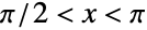 で
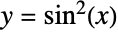 を
 軸について回転させることで包み込まれる体積を計算する:
Integrate[π(Sin[x] ^ 2) ^ 2, {x, 0, π}]RevolutionPlot3D[Sin[x] ^ 2, {x, 0, π}, RevolutionAxis -> "X"]円筒形の外殻を使って,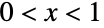 で
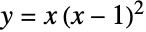 を
 軸に沿って回転することで包み込まれる体積を求める:
Integrate[2π x(x(x - 1) ^ 2), {x, 0, 1}]
Show[RevolutionPlot3D[{x(x - 1) ^ 2}, {x, 0, 1}], RevolutionPlot3D[0, {x, 0, 1}]] 軸の周りで
 と
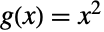 の間の面を回転させることで生成される領域の体積を求める:
f[x_] := x
g[x_] := x^2Solve[f[x] == g[x], x]


Plot[{g[x], f[x]}, {x, 0, 1}, Filling -> {2 -> {1}}]RevolutionPlot3D[{{x, f[x]}, {x, g[x]}}, {x, 0, 1}, PlotStyle -> Opacity[.6]]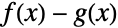

Subsuperscript[∫, 0, 1]2π x(f[x] - g[x])ⅆx の上で
 の下の領域を
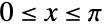 の範囲で
 軸の周りで回転させた体積を求める:
f[x_] := Csc[x]
Solve[f[x] == 2 && 0 ≤ x ≤ π, x]
Plot[{2, f[x]}, {x, 0, π}, Filling -> {2 -> {1}}, PlotRange -> {0, 2}]Show[RevolutionPlot3D[f[x], {x, (π/6), (5 π/6)}, RevolutionAxis -> {1, 0, 0}], Graphics3D[{Opacity[.5], Cylinder[{{0, 0, 0}, {π, 0, 0}}, 2]}], ViewPoint -> {2, -2.5, 1}, PlotRange -> {{π / 6, 5π / 6}, {-2, 2}, {-2, 2}}]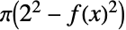
Subsuperscript[∫, (π/6), (5 π/6)]π(2^2 - f[x]^2)ⅆx%//N 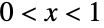 の範囲で
 を
 軸に沿って回転したときの曲面の面積を計算する:
RevolutionPlot3D[x ^ 3, {x, 0, 1}]w = Sqrt[1 + D[x ^ 3, x] ^ 2]
Subsuperscript[∫, 0, 1]2 π x wⅆx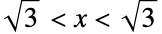
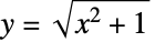

RevolutionPlot3D[Sqrt[x^2 + 1], {x, -Sqrt[3], Sqrt[3]}, RevolutionAxis -> "X"]w = Sqrt[1 + D[Sqrt[x ^ 2 + 1], x]^2]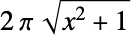
Subsuperscript[∫, -Sqrt[3], Sqrt[3]]2 π Sqrt[x^2 + 1] wⅆx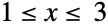


f[x_] := 1 / xw = Sqrt[1 + D[f[x], x]^2]


Subsuperscript[∫, 1, 3]2π(4 - x)wⅆx%//N//Chop直線  および
 に基づいた修正円筒座標を使って曲面を可視化する:
ParametricPlot3D[{Cos[θ](x - 4) + 4, 1 / x, Sin[θ](x - 4)}, {x, 1, 3}, {θ, 0, 2π}, IconizedObject[«ParametricPlot3D options»]]弧長,曲面の面積,および体積 (8)
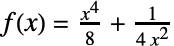


f[x_] := (x^4/8) + (1/4 x^2)Plot[f[x], {x, 1, 2}, PlotRange -> {0, 2}]ds = Sqrt[1 + D[f[x], x] ^ 2]//SimplifyIntegrate[ds, {x, 1, 2}]ArcLengthが返す答と比較する:
ArcLength[f[x], {x, 1, 2}]


f[x_] := Sqrt[x - x^2] + ArcSin[Sqrt[x]]Plot[f[x], {x, 0, 1}]ds = Sqrt[1 + D[f[x], x] ^ 2]//SimplifyIntegrate[ds, {x, 0, 1}]ArcLengthが返した答と比較する:
ArcLength[f[x], {x, 0, 1}]{x, y} = {2Cos[u], 2Sin[u]};

ParametricPlot[{x, y}, {u, 0, 2π}]ds = Sqrt[D[x, u] ^ 2 + D[y, u] ^ 2]//SimplifyIntegrate[ds, {u, 0, 2π}]ArcLengthが返す答と比較する:
ArcLength[{x, y}, {u, 0, 2π}]c[u_] = {1, 0, 0}2Cos[u] + Normalize[{0, 1, 1}]Sin[u]ParametricPlot3D[c[u], {u, 0, 2π}]ds = Sqrt[c'[u].c'[u]]Integrate[ds, {u, 0, 2π}]%//NArcLengthが返す答と比較する:
ArcLength[c[u], {u, 0, 2π}]

f[x_, y_] := x^2 + y^2Plot3D[f[x, y], {x, 0, 1}, {y, 0, 1}, BoxRatios -> Automatic]dA = Sqrt[1 + D[f[x, y], x] ^ 2 + D[f[x, y], y] ^ 2]//SimplifyIntegrate[dA, {x, 0, 1}, {y, 0, 1}]%//NAreaが返す答と比較する:
Area[f[x, y], {x, 0, 1}, {y, 0, 1}]

s[u_, v_] := {(2 + Cos[v])Cos[u], (2 + Cos[v])Sin[u], Sin[v]}ParametricPlot3D[s[u, v], {u, 0, 2π}, {v, 0, 2π}]dA = Simplify[Norm[Subscript[∂, u]s[u, v]⨯Subscript[∂, v]s[u, v]], {u, v}∈ℝ]Integrate[dA, {u, 0, 2π}, {v, 0, 2π}]Areaが返す答と比較する:
Area[s[u, v], {u, 0, 2π}, {v, 0, 2π}]以下のパラメトリック領域の体積を求める.ただし,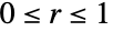 ,
 である:
ρ[r_, u_, v_] := {(2 + r Cos[v])Cos[u], (2 + r Cos[v])Sin[u], Sin[v]}ParametricPlot3D[ρ[1, u, v], {u, 0, 2Pi}, {v, 0, 2Pi}]j = Simplify[RealAbs[Det[Grad[ρ[r, u, v], {r, u, v}]]], 0 ≤ r ≤ 1 && 0 ≤ v ≤ 2π]Subsuperscript[∫, 0, 1]Subsuperscript[∫, 0, 2 π]Subsuperscript[∫, 0, 2π]jⅆuⅆvⅆrVolumeが返す答と比較する:
Volume[ρ[r, u, v], {r, 0, 1}, {u, 0, 2Pi}, {v, 0, 2Pi}]以下のパラメトリック領域の体積を求める.ただし,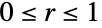 ,
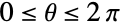 ,
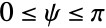 である:
ρ[r_, θ_, ψ_] := {3r Cos[ψ], 2r Sin[θ]Sin[ψ], r Cos[θ]Sin[ψ]}ParametricPlot3D[ρ[1, θ, ψ], {θ, 0, 2Pi}, {ψ, 0, Pi}]j = Simplify[RealAbs[Det[Grad[ρ[r, θ, ψ], {r, θ, ψ}]]], 0 ≤ r ≤ 1 && 0 ≤ ψ ≤ π]Subsuperscript[∫, 0, 1]Subsuperscript[∫, 0, 2 π]Subsuperscript[∫, 0, π]jⅆψⅆθⅆrVolumeが返す答と比較する:
Volume[ρ[r, θ, ψ], {r, 0, 1}, {θ, 0, 2Pi}, {ψ, 0, Pi}]線積分 (6)
原点を中心とした半長軸が と
 の楕円上で
 の線形積分
 を計算する:
f[{x_, y_}] := x + y^2reg = Region[Circle[{0, 0}, {2, 1}], Axes -> True]c[t_] := {2Cos[t], Sin[t]}ParametricPlot[c[t], {t, 0, 2Pi}]
Subsuperscript[∫, 0, 2 π]f[c[t]] Norm[Derivative[1][c][t]]ⅆt%//NUnderscript[∫, 𝕩∈reg]f[𝕩]以下のパラメータ化された曲線上で  の閉じた線形積分
 を計算する:
c[t_] := {Cos[t], Sin[2t]}この曲線は,以下のプロットで示されているように,赤から紫に進む無限大の形を形成する:
Show[ParametricPlot[{Cos[x], Sin[2x]}, {x, 0, 2Pi}, PlotTheme -> "Detailed", ColorFunction -> (Hue[0.8#3]&)]]
v[{x_, y_}] := {x y, 3y ^ 2}
Integrate[v[c[t]].c'[t], {t, 0, 2π}]頂点 ,
 ,
 の三角形上で ∫x4dx+x yyを計算するために,関連するベクトル場を定義する:
v[{x_, y_}] := {x^4, x y}c[t_] = Piecewise[{{{0, 0} + t*({1, 0} - {0, 0}), 0 <= t <= 1}, {{1, 0} + (t - 1)*({0, 1} - {1, 0}),
1 <= t <= 2}, {{0, 1} + (t - 2)*({0, 0} - {0, 1}), 2 <= t <= 3}, {Indeterminate, True}}]ParametricPlot[c[t], {t, 0, 3}, PlotTheme -> "FrameGrid", ColorFunction -> (Hue[0.8#3]&)]
Integrate[v[c[t]].c'[t], {t, 0, 3}]粒子が (
 )から
 (
 )までの以下のパスを通るときの,力
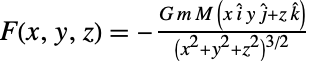 によってなされた仕事を計算する:
c[t_] := {a Cos[t], b Sin[t], t(t - Pi / 2)}F[{x_, y_, z_}] := -(G M m{x, y, z}/(x^2 + y^2 + z^2)^3 / 2)
Integrate[F[c[t]].c'[t], {t, 0, Pi / 2}, Assumptions -> {a > 0, b > 0}]//Expandv[{x_, y_, z_}] := {x ^ 2, y ^ 2, z ^ 2}Curl[v[{x, y, z}], {x, y, z}]時点 における原点から時点
 における
 まで進む,直線を通る曲線の族を定義する:
Subscript[c, {x_, y_, z_}][t_] := t{x, y, z}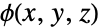


ϕ[{x_, y_, z_}] = Subsuperscript[∫, 0, 1]v[Subscript[c, {x, y, z}][t]].D[Subscript[c, {x, y, z}][t], t]ⅆtGradを使って  が
 のポテンシャル関数であることを確認する:
Grad[ϕ[{x, y, z}], {x, y, z}] == v[{x, y, z}]グリーンの定理(Green's Theorem) を使って次の曲線で囲まれた部分の面積を求める:
c[u_] := {Cos[u] + 1 / 7Cos[7u + π / 3], Sin[u] + 1 / 7Sin[7u]};ParametricPlot[c[u], {u, 0, 2π}]次のベクトル場は の二次元Curlを持つ:
v[{x_, y_}] := {0, x}Curl[v[{x, y}], {x, y}]
Subsuperscript[∫, 0, 2 π]v[c[u]].Derivative[1][c][u]ⅆu曲面と体積の積分 (7)
グリーンの定理を使って,原点を中心として半径3の円の上で  を計算する:
v[x_, y_] := {3y^3 - Exp[Sin[x]], 7x^2 + Sqrt[y^4 + 1]}VectorPlot[v[x, y], {x, -3, 3}, {y, -3, 3}, Epilog -> Circle[{0, 0}, 3], PlotRangePadding -> None]ベクトル場の循環はCurlを使って行うことができる:
circ = Curl[v[x, y], {x, y}]Subsuperscript[∫, -3, 3]Subsuperscript[∫, -Sqrt[9 - y^2], Sqrt[9 - y^2]]circⅆxⅆyUnderscript[∫, {x, y}∈Disk[{0, 0}, 3]]circ
f[{x_, y_, z_}] := (x + y + z)^4s[θ_, φ_] := {Sin[θ]Cos[φ], Sin[θ]Sin[φ], Cos[θ]}dS = Simplify[Norm[Subscript[∂, θ]s[θ, φ]⨯Subscript[∂, φ]s[θ, φ]], 0 ≤ θ ≤ π && -π < φ < π]
Subsuperscript[∫, 0, 2π]Subsuperscript[∫, 0, π]f[s[θ, φ]]dSⅆθⅆφSubscript[∫, 𝕏∈Sphere[]]f[𝕏]
v[{x_, y_, z_}] := {-y, x, x ^ 2 - y ^ 2}s[u_, v_] := {Sin[u]Cos[v], Sin[u]Sin[v], Cos[u]}Show[ParametricPlot3D[s[u, v], {u, 0, Pi / 2}, {v, 0, 2Pi}], VectorPlot3D[v[{x, y, z}], {x, -1, 1}, {y, -1, 1}, {z, 0, 1}], PlotRange -> {{-1, 1}, {-1, 1}, {0, 1}}]
c[t_] := {Cos[t], Sin[t], 0}curl[{x_, y_, z_}] = Curl[v[{x, y, z}], {x, y, z}]dS = Subscript[∂, u]s[u, v]⨯Subscript[∂, v]s[u, v]//SimplifyStokeの定理  には,境界上の
 の線形積分は曲面を通るその回転の流束積分に等しいとある:
Subsuperscript[∫, 0, (π/2)]Subsuperscript[∫, 0, 2 π]curl[s[u, v]].dSⅆvⅆu == Subsuperscript[∫, 0, 2 π]v[c[t]].Derivative[1][c][t]ⅆt発散定理を使って,上界が 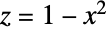 .下界が
 で両側の境界が
 と
 である曲面を通る
 の流束を計算する:
ContourPlot3D[{y + z == 2, z == 1 - x ^ 2, z == 0, y == 0}, {x, -1.5, 1.5}, {y, 0, 2}, {z, 0, 1}, ContourStyle -> Opacity[0.5], Mesh -> None]
Subsuperscript[∫, -1, 1]Subsuperscript[∫, 0, 1 - x^2]Subsuperscript[∫, 0, 2 - z]Div[{x y, y^2 + E^x z^2, Sin[x y]}, {x, y, z}]ⅆyⅆzⅆxガウス定理を使って以下のパラメトリック曲面で包み込まれた部分の体積を求める:
s[u_, v_] := {(2 + Cos[v])Cos[u], (2 + Cos[v])Sin[u], Sin[v](5 / 4 - Cos[u])}ParametricPlot3D[s[u, v], {u, 0, 2π}, {v, 0, 2π}]dA = Subscript[∂, u]s[u, v]⨯Subscript[∂, v]s[u, v]//FullSimplify
v[{x_, y_, z_}] := (1/3){x, y, z}Div[v[{x, y, z}], {x, y, z}]
Integrate[v[s[u, v]].dA, {u, 0, 2π}, {v, 0, 2π}]質量密度  が与えられた場合に,以下で与えられる領域の質量を求める:
φ[u_, v_, w_] := {(5 + 2w Cos[v])Cos[u], 2Sin[v], (5 + 2w Cos[v])Sin[u]};塗り潰されたトーラスを生成するパラメータの範囲は  および
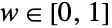 である:
ParametricPlot3D[φ[u, v, 1], {u, 0, 2π}, {v, 0, 2π}]ρ[{x_, y_, z_}] := (2 - y^2)(x^2 + z^2)jac = Simplify[RealAbs@Det[Grad[φ[u, v, w], {u, v, w}]], 0 ≤ w ≤ 1 && v∈Reals]Integrate[ρ[φ[u, v, w]]jac, {u, 0, 2π}, {v, 0, 2π}, {w, 0, 1}]

Table[Integrate[Sum[Indexed[x, i] ^ 2, {i, n}], x∈Ball[n]], {n, 10}]FindSequenceFunction[%, n]Table[(n π^n / 2/2 Gamma[2 + (n/2)]), {n, 10}]平均値と重心 (6)



(Subsuperscript[∫, 0, π]Cos[x]^4 Sin[x]ⅆx/π - 0)Plot[{Cos[x] ^ 4Sin[x], 2 / (5π)}, {x, 0, π}]


reg = Region[Parallelogram[{0, 0}, {{1, 0}, {1, 2}}], ImageSize -> Small, Axes -> True]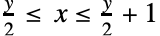
(Integrate[x + y, {y, 0, 2}, {x, y / 2, y / 2 + 1}]/Integrate[1, {y, 0, 2}, {x, y / 2, y / 2 + 1}])(Integrate[x + y, {x, y}∈reg]/Area[reg])Plot3D[{x + y, 2}, {x, y}∈reg, BoxRatios -> {1, 1, 1}] から
 までの曲線
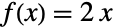 の下の領域の重心を計算するために,まず 面積を求める:
a = Integrate[2x, {x, 0, 1}]xcentroid = (1 / a)Integrate[x, {x, 0, 1}, {y, 0, 2x}]ycentroid = (1 / a)Integrate[y, {x, 0, 1}, {y, 0, 2x}]RegionCentroidが与える答と比較する:
p = RegionCentroid[ImplicitRegion[0 ≤ y ≤ 2x && 0 ≤ x ≤ 1, {x, y}]]Show[Plot[2x, {x, 0, 1}, Filling -> Axis], Graphics[{PointSize[Large], Point[p]}]]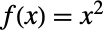
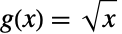


a = Integrate[Sqrt[x] - x ^ 2, {x, 0, 1}]xcentroid = (1 / a)Integrate[x(Sqrt[x] - x ^ 2), {x, 0, 1}]ycentroid = (1 / a)Integrate[(1 / 2)((Sqrt[x]) ^ 2 - (x ^ 2) ^ 2), {x, 0, 1}]RegionCentroidが返す答と比較する:
p = RegionCentroid[ImplicitRegion[x ^ 2 ≤ y ≤ Sqrt[x] && 0 ≤ x ≤ 1, {x, y}]]Show[Plot[{x ^ 2, Sqrt[x]}, {x, 0, 1}, Filling -> {1 -> {2}}, PlotLegends -> "Expressions"], Graphics[{PointSize[Large], Point[p]}]]曲線 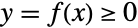 の下の
 から
 までの領域の重心の一般式を,積分は曲線の下の面積を与えるという事実を使って導出する:
A = Subsuperscript[∫, a, b]f[x]ⅆx; の重心は,
 から
 までと
 から
 までの領域上の
 の平均値である:
(1/A)Subsuperscript[∫, a, b]Subsuperscript[∫, 0, f[x]]xⅆyⅆx

(1/A)Subsuperscript[∫, a, b]Subsuperscript[∫, 0, f[x]]yⅆyⅆx

reg = Region[ImplicitRegion[x ^ 2 + y ^ 2 + z ^ 2 ≤ 3 && y ≥ 0, {x, y, z}]]v = Integrate[1, 𝕏∈reg]cm = (1/v)Integrate[𝕏, 𝕏∈reg]Show[RegionPlot3D[DiscretizeRegion@reg, Mesh -> None, Axes -> True, PlotStyle -> Opacity[1 / 2]], Graphics3D[{StandardCyan, Sphere[cm, 0.1]}]]確率,期待値,標準偏差 (7)

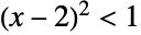
pdf = PDF[NormalDistribution[0, 1], x]Integrate[Boole[(x - 2) ^ 2 < 1]pdf, {x, -∞, ∞}]Probabilityが返す値と比較する:
Probability[(x - 2) ^ 2 < 1, xNormalDistribution[0, 1]]平均 の指数分布について
 の確率を計算する.平均はパラメータの逆数である:
Mean[ExponentialDistribution[μ]]したがって,ExponentialDistribution[5/2]の確率密度関数(PDF)を使用する:
PDF[ExponentialDistribution[(5/2)], x]
Integrate[(5 / 2)E ^ (-5t / 2), {t, 4, ∞}]PDFは  の場合に消失するため,
 である確率は,
 から
 までの積分で与えられる:
Integrate[(5 / 2)E ^ (-5t / 2), {t, 0, 2}]Probability[x > 4, xExponentialDistribution[5 / 2]]Probability[x < 2, xExponentialDistribution[5 / 2]]//Expand(1/σ Sqrt[2 π])Subsuperscript[∫, μ - 2 σ, μ + 2 σ]Exp[-((x - μ)^2/2 σ^2)]ⅆxProbabilityが返す答と比較する:
Probability[μ - 2σ ≤ x ≤ μ + 2σ, xNormalDistribution[μ, σ]]
N[Erf[Sqrt[2]]]これは,曲線の下の面積全体の が,以下のプロットで
 と
 の間にあると解釈できる:
p[x_] = PDF[NormalDistribution[0, 1], x];
tr[x_] = Piecewise[{{p[x], -2 <= x <= 2}, {Indeterminate, True}}];
Plot[{p[x], tr[x]}, {x, -3, 3}, Filling -> Axis, AxesLabel -> {x / σ, p}]

pdf = PDF[CauchyDistribution[0, 1], x]Integrate[Sqrt[Abs[x]] pdf, {x, -∞, ∞}]Expectationが返す答と比較する:
Expectation[Sqrt[Abs[x]], xCauchyDistribution[0, 1]]Integrate[x PDF[NormalDistribution[μ, σ], x], {x, -∞, ∞}, Assumptions -> σ > 0]Integrate[(x - μ) ^ 2PDF[NormalDistribution[μ, σ], x], {x, -∞, ∞}, Assumptions -> σ > 0]{Mean[NormalDistribution[μ, σ]], Variance[NormalDistribution[μ, σ]]}平均の μ 指数分布の標準偏差はやはり μ であることを示す:
Refine[Sqrt[(1/μ)Subsuperscript[∫, 0, ∞]E^-x / μ(x - μ)^2ⅆx], μ > 0]MeanとStandardDeviationが返す答と比較する:
dist = ExponentialDistribution[1 / μ];{Mean[dist], StandardDeviation[dist]}確率密度関数(PDF)から累積分布関数(CDF)を計算する:
pdf[x_] = PDF[NormalDistribution[0, 1], x]cdf[x_] = Integrate[pdf[x], {x, -∞, x}]累積分布関数は, から
 までの確率密度関数曲線の下の面積を与える:
Manipulate[Plot[{pdf[x], cdf[x]}, {x, -3, u}, Filling -> {1 -> Axis}, PlotTheme -> "Detailed", PlotRange -> {{-3, 3}, {0, 1}}, PlotLabel -> x == u], {{u, 0, x}, -3.01, 3}, SaveDefinitions -> True]積分変換 (7)
ft[f_, x_, ω_] := (1/Sqrt[2π])Integrate[f Exp[I ω x], {x, -∞, ∞}]ft[Exp[-x ^ 2], x, ω]FourierTransformと比較する:
FourierTransform[Exp[-x ^ 2], x, ω]lt[f_, x_, s_] := Integrate[f Exp[-s x], {x, 0, ∞}]lt[x ^ 2, x, s]LaplaceTransformと比較する:
LaplaceTransform[x ^ 2, x, s]ht[f_, x_, ω_] := (1/Sqrt[2π])Integrate[f(Cos[ω x] + Sin[ω x]), {x, -∞, ∞}]ht[Exp[-x ^ 2], x, ω]この関数は偶関数なので,Hartley変換はFourierCosTransformに等しい:
FourierCosTransform[Exp[-x ^ 2], x, ω]a[0] = 2Integrate[x^2, {x, 0, 1}]a[i_] = 2Integrate[x^2 Cos[2π i x], {x, 0, 1}, Assumptions -> i∈ℤ]b[i_] = 2Integrate[x^2 Sin[2π i x], {x, 0, 1}]s[n_] := a[0] / 2 + Subsuperscript[∑, i = 1, n]a[i]Cos[2π i x] + Subsuperscript[∑, i = 1, n]b[i]Sin[2π i x]
Plot[{x ^ 2, s[#]}, {x, 0, 1}, PlotTheme -> {"Minimal"}, PlotLabel -> n == #, ImageSize -> 225]& /@ Range[2, 8, 2]mt[f_, x_, s_] := Integrate[f x ^ (s - 1), {x, 0, ∞}]mt[Sin[x], x, s]MellinTransformと比較する:
MellinTransform[Sin[x], x, s, GenerateConditions -> True]ht[f_, r_, s_, ν_] := Integrate[r f BesselJ[ν, r s], {r, 0, ∞}, Assumptions -> s > 0 && ν > -1 / 2]ht[1 / r, r, s, 0]HankelTransformと比較する:
HankelTransform[1 / r, r, s, ν]fract[α_, w_] = Sqrt[(1 - I Cot[α]) / (2π)]E ^ (I Cot[α] w ^ 2 / 2) Integrate[E ^ (-I Csc[α] w t + I Cot[α] t ^ 2 / 2) UnitBox[t], {t, -∞, ∞}]Table[Plot[{Re[fract[α, w]], Im[fract[α, w]]}, {w, -2, 2}, Filling -> Axis, PlotRange -> All, ImageSize -> 225, PlotLabel -> α == α], {α, {0.02π, 0.09π, 3.2π, 20.9π}}]実部と虚部の解析 (4)

lp[p_, f_, x_] := Integrate[Abs[f] ^ p, {x, -∞, ∞}, Assumptions -> p ≥ 1] ^ (1 / p)Format[HoldPattern[lp[p_, f_, x_]]] := HoldForm[Norm[f, L^p]]
f := Exp[-x^2];
g := Exp[-5 x^2];
h := HeavisideTheta[x] Exp[-5 x^2];{lp[p, f, x], lp[p, g, x], lp[p, h, x]}ノルムは常に最終的に  の増加関数であるが,はじめは減少するかもしれない:
Plot[{lp[p, f, x], lp[p, g, x], lp[p, h, x]}, {p, 1, 12}, PlotTheme -> "Detailed", Evaluated -> True, PlotRange -> All]フーリエ変換は  同型(関数のノルムと変換したもののノルムは等しい)である:
Table[lp[2, fn, x] == lp[2, FourierTransform[fn, x, k], k], {fn, {f, g}}]//FullSimplify

Table[lp[1, fn, x] == lp[1, FourierTransform[fn, x, k], k], {fn, {f, g, h}}]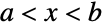 で定義された関数について,重み
 で
 の重み付き内積を定義する:
ip[w_, f_, g_, {x_, a_, b_}] := Integrate[w f Conjugate[g], {x, a, b}]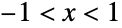

Table[ip[1, LegendreP[n, x], LegendreP[m, x], {x, -1, 1}], {n, 0, 4}, {m, 0, 4}]//MatrixForm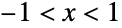


Table[ip[(1/Sqrt[1 - x ^ 2]), ChebyshevT[n, x], ChebyshevT[m, x], {x, -1, 1}], {n, 0, 4}, {m, 0, 4}]//MatrixForm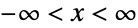


Table[ip[Exp[-x ^ 2], HermiteH[n, x], HermiteH[m, x], {x, -∞, ∞}], {n, 0, 4}, {m, 0, 4}]//MatrixFormIntegrateを使って関数の内積を定義する:
dot[f_, g_] := (2/π)Subsuperscript[∫, -1, 1]Conjugate[f]gSqrt[1 - x^2]ⅆxOrthogonalizeを使って正規直交基底を構築する:
Orthogonalize[{1, x, x^2, x^3, x^4}, dot]//Expand内積はゲーゲンバウアー(Gegenbauer)多項式を生成する:
Table[GegenbauerC[n, 1, x], {n, 0, 4}] における
 の剰余を,
 を包み込む輪郭線上での積分として計算する:
res[f_, {z_, c_}] := Underscript[, r -> 0^ + ](1/2 π I)Subsuperscript[∫, 0, 2 π](f Dt[z, t] /. z -> c + Exp[I t])ⅆtres[(2/z - 1), {z, 1}]res[(Sin[z]/(z - 2) ^ 3), {z, 2}]Residueが返す答と比較する:
Residue[(2/z - 1), {z, 1}]Residue[(Sin[z]/(z - 2) ^ 3), {z, 2}]特殊関数の積分表現 (3)
Assuming[{Re[z] > 0, n∈ℤ}, FullSimplify[HermiteH[n, z] == (2^n Subsuperscript[∫, -∞, ∞]((z + I t)^n/E^t^2)ⅆt/Sqrt[π])]]Plot[Table[HermiteH[n, z], {n, 0, 4}]//Evaluate, {z, 0, 4}, PlotTheme -> {"Detailed", "DashedLines"}]Gammaを対数積分によって表す:
Simplify[Gamma[z] == Integrate[Log[1 / t] ^ (z - 1), {t, 0, 1}], Re[z] > 0]Plot[Gamma[z], {z, 0, 5}]FullSimplify[Zeta[s] == (1/Gamma[s])Subsuperscript[∫, 0, ∞](t^s - 1/E^t - 1)ⅆt, Re[s] > 1]特性と関係 (14)
f[x_] = E ^ x;g[x_] = x ^ 2 + 4x + 17;∫(f[x] + b g[x])ⅆx == ∫f[x]ⅆx + b ∫g[x]ⅆx//Simplifyf[x_] := x ^ n + x ^ -nIntegrate[f[x], x]f[x] == D[%, x]定積分はDiscreteLimitとSumによって定義できる:
f[x_] := 1 / xSubsuperscript[∫, 1, 3]f[x]ⅆx == Underscript[, nUnderscript[ -> , ℤ]∞]Underoverscript[∑, k = 0, n - 1]f[1 + k((3 - 1)/n)](3 - 1/n)Nを使って積分を数値的に評価する:
Integrate[Sin[Sin[x]], {x, 0, 1}]N[%]これは,事実上,NIntegrateを呼び出す:
NIntegrate[Sin[Sin[x]], {x, 0, 1}]負の整数次数を持つDerivativeは積分を行う:
Derivative[-2][Function[x, x ^ n]][x]Integrate[x ^ n, x, x]//FactorArcLengthは,一次元領域上での1の積分である:
Underscript[∫, {x, y}∈Circle[]]1ArcLength[Circle[]]Areaは,二次元領域上での1の積分である:
Underscript[∫, {x, y, z}∈Sphere[]]1Area[Sphere[]]Volumeは,三次元領域上での1の積分である:
Underscript[∫, {x, y, z}∈Ball[]]1Volume[Ball[]]領域  についてのRegionMeasureは積分
 で与えられる:
ℛ = Circle[];{RegionMeasure[ℛ], Integrate[1, {x, y}∈ℛ]}ℛ = Ball[];{RegionMeasure[ℛ], Integrate[1, {x, y, z}∈ℛ]}RegionCentroidは,m=RegionMeasure[ℛ]のIntegrate[p,p∈ℛ]/m に等しい:
ℛ = Sphere[{1, 2, 3}];
m = RegionMeasure[ℛ];{RegionCentroid[ℛ], Integrate[p, p∈ℛ] / m}Integrate[Sin[x], x]DSolveValueは積分定数を持つ解を返す:
DSolveValue[y'[x] == Sin[x], y[x], x]DSolveは解の置換規則を返す:
DSolve[y'[x] == Sin[x], y, x]Integrateは積分を閉形式で計算する:
closed = Integrate[Sin[x t] ^ 2, {t, 0, 1}]AsymptoticIntegrateは厳密解を近似する級数を与える:
AsymptoticIntegrate[Sin[x t] ^ 2, {t, 0, 1}, {x, 0, 8}]Series[closed, {x, 0, 8}]//NormalFourierTransformは積分によって定義される:
FourierTransform[Exp[-t ^ 2] Sin[t], t, ω] == Subsuperscript[∫, -∞, ∞]Exp[-t^2] Sin[t]( Exp[I ω t]/Sqrt[2 π])ⅆt//SimplifyLaplaceTransformは積分によって定義される:
LaplaceTransform[Exp[-t ^ 2] Sin[t], t, s] == Subsuperscript[∫, 0, ∞]Exp[-t^2] Sin[t] Exp[-s t]ⅆt//FullSimplify考えられる問題 (13)
不定積分 (6)
単純な積分の中にも標準的な数学関数で評価できないものがたくさんある:
Integrate[Sin[x] / Log[x], x]f[x_] := 1 / (2 + Sin[x])Plot[{f[x], Integrate[f[x], x]}, {x, 0, 2π}, PlotTheme -> "Detailed", Evaluated -> True]定積分を可変上界で使うと不連続なところが滑らかになる.プロットの左側の不連続点を求める:
Solve[Integrate[f[x], x] == 0 && -π < x < 0, x]この場合,前の不連続点から積分することにより,不定積分の値が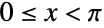 の範囲で再現される:
Assuming[{x∈Reals}, Plot[{f[x], Integrate[f[t], {t, -2 ArcTan[(1/2)], x}]}, {x, 0, 2π}, PlotTheme -> "Detailed", Evaluated -> True, Filling -> {1 -> 0}]]Integrate[1 / Sqrt[a^2 - x ^ 2], x]D[%, x]Simplifyおよび関連構造はしばしば同値を示す:
Simplify[%]同じ被積分関数でも形式が異なると積分定数が異なる積分を与えることがある:
Integrate[1 + (x + 1) ^ 3, x]Integrate[Expand[1 + (x + 1) ^ 3], x]Simplify[%% - %] のようなパラメータは不定積分の内側では汎用的であると仮定される:
Integrate[x ^ n, x]Integrate[x ^ -1, x]Integrate[t ^ n, {t, 0, x}]和の一部が明示的に積分できなければ,和全体が積分されずに残される:
Integrate[f[x] + f'[x], x]Integrate[f[x], x] + Integrate[f'[x], x]定積分 (7)
不定積分の結果に上界下界を代入することでは定積分の正しい答が得られないかもしれない:
Integrate[1 / (2 + Cos[x]), {x, 0, 2π}]expr = Integrate[1 / (2 + Cos[x]), x](expr /. x -> 2π) - (expr /. x -> 0)Plot[expr, {x, 0, 2π}]整数による仮定を指定してもより簡単な結果が与えられるとは限らない:
Integrate[k Cos[k x], {x, -π, π}, Assumptions -> k∈Integers]Simplifyおよび関連関数を使って望んだ結果を得る:
Simplify[%, k∈Integers]Integrate[Exp[-x] LaguerreL[n, x] ^ 2, {x, 0, Infinity}, Assumptions -> Element[n, PositiveReals]]
NIntegrate[Exp[-x] LaguerreL[Pi, x] ^ 2, {x, 0, Infinity}]
Integrate[Exp[-x] LaguerreL[3, x] ^ 2, {x, 0, Infinity}]整数性等の離散サブケースの指定でも,一般的な結果が得られる:
Integrate[Exp[-x] LaguerreL[n, x] ^ 2, {x, 0, Infinity}, Assumptions -> Element[n, PositiveIntegers]]
Integrate[BesselJ[2, x] / (1 + x ^ 2), {x, 0, 1}]Integrate[BesselJ[2, x] / (1 + x ^ 2), {x, 0, ∞}]領域上の積分は,被積分関数が絶対に積分可能かどうかを調べはしない:
Integrate[(x^2 - y^2/(x^2 + y^2)^2), {x, y}∈Rectangle[{0, 0}, {1, 1}]]Underscript[, a -> 0^ + ]Integrate[Abs[(x^2 - y^2/(x^2 + y^2)^2)], {x, y}∈Rectangle[{a, a}, {1, 1}]]Integrate[(x ^ 2 - y ^ 2) / (x ^ 2 + y ^ 2) ^ 2, {x, 0, 1}, {y, 0, 1}]Integrate[(x ^ 2 - y ^ 2) / (x ^ 2 + y ^ 2) ^ 2, {y, 0, 1}, {x, 0, 1}]ℛ = RegionIntersection[Ball[{0, 0, 0}, Sqrt[14]], Ball[{2, 4, 6}, Sqrt[14]]]Integrate[x + y + z, {x, y, z}∈ℛ]全空間の測度を使う場合は,条件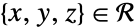 を加えて空間全体の上で積分する:
Integrate[(x + y + z) Boole[{x, y, z}∈ℛ], {x, y, z}∈FullRegion[3]]GenerateConditionsをFalseに設定すると予想しない答が返されるかもしれない:
Integrate[1 / x, {x, 0, a}, GenerateConditions -> False]Integrate[1 / x, {x, 0, a}]
インタラクティブな例題 (1)
 のとき,
 を
 軸の周りで回転させた内部であるガブリエルのラッパについて考える:
f[x_] := 1 / x
v[a_] = Integrate[π f[x] ^ 2, {x, 1, a}, Assumptions -> a > 1]
s[a_] = Integrate[2π f[x]Sqrt[1 + D[f[x], x] ^ 2], {x, 1, a}, Assumptions -> a > 1]
Underscript[, a -> ∞]{v[a], s[a]}ラッパを, の関数としてのその体積と表面積とともに可視化する:
Manipulate[Column[{Style[a == b//TraditionalForm, FontSize -> 14], RevolutionPlot3D[1 / s, {s, 1, b}, RevolutionAxis -> {1, 0, 0}, PlotRange -> {{1, 15}, {-1, 1}, {-1, 1}}, Mesh -> None, ImageSize -> 300, Ticks -> None, Boxed -> False], Show[Plot[{s[x], v[x]}, {x, 1, 16}, ImageSize -> Small, PlotLegends -> {"Surface Area" == NumberForm[s[b], {5, 3}], "Volume" == NumberForm[v[b], {4, 3}]}], Graphics[{StandardOrange, PointSize[Large], Point[{b, v[b]}], StandardBlue, Point[{b, s[b]}]}]]}, Alignment -> Center], {{b, 5., a}, 1.01, 15}, SaveDefinitions -> True]おもしろい例題 (2)
最初の6つのボールウェイン(Borwein)型の積分は,すべて厳密に である:
Table[Subsuperscript[∫, 0, ∞](Underoverscript[∏, k = 0, max](Sin[(x/2 k + 1)]/(x/2 k + 1)))ⅆx, {max, 6}]7番目からは,少しずつ からずれる.例えば,8番目は以下のようになる:
Subsuperscript[∫, 0, ∞](Underoverscript[∏, k = 0, 8](Sin[(x/2 k + 1)]/(x/2 k + 1)))ⅆxN[% - Pi / 2]シュリニヴァーサ・ラマヌジャン(Srinivasa Ramanujan)のノートにあった対数積分:
Integrate[Log[(1 + Sqrt[1 + 4x]) / 2] / x, {x, 0, 1}]
 MathWorld

 NKS|Online
テキスト
Wolfram Research (1988), Integrate, Wolfram言語関数, https://reference.wolfram.com/language/ref/Integrate.html (2026年に更新).
CMS
Wolfram Language. 1988. "Integrate." Wolfram Language & System Documentation Center. Wolfram Research. Last Modified 2026. https://reference.wolfram.com/language/ref/Integrate.html.
APA
Wolfram Language. (1988). Integrate. Wolfram Language & System Documentation Center. Retrieved from https://reference.wolfram.com/language/ref/Integrate.html