


ListSliceVectorPlot3D
ListSliceVectorPlot3D[varr,surf]
generates a vector plot from a 3D array varr of vector field values over the slice surface surf.
ListSliceVectorPlot3D[…,{surf1,surf2,…}]
generates a slice vector plot over several surfaces surf1, surf2, ….
Details and Options
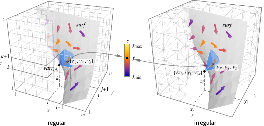
- ListSliceVectorPlot3D evaluates the interpolated field function
 at values of x, y and z on a surface surf and displays the results as arrows colored by magnitude.
 - For regular data, the field function
 has value varr[[i,j,k]] at
  .
. - For irregular data,
 has value {vxi,vyi,vzi} at
  .
. - The plot visualizes the set
 where region reg is the Cartesian product
  for regular data and the convex hull of {{x1,y1,z1},…,{xn,yn,zn}} for irregular data.
 - The following basic slice surfaces surfi can be given:
-
Automatic automatically determine slice surfaces 
"CenterPlanes" coordinate planes through the center 
"BackPlanes" coordinate planes at the back of the plot 
"XStackedPlanes" coordinate planes stacked along  axis
axis
"YStackedPlanes" coordinate planes stacked along  axis
axis
"ZStackedPlanes" coordinate planes stacked along  axis
axis
"DiagonalStackedPlanes" planes stacked diagonally 
"CenterSphere" a sphere in the center 
"CenterCutSphere" a sphere with a cutout wedge 
"CenterCutBox" a box with a cutout octant - ListSliceVectorPlot3D[data] is equivalent to ListSliceVectorPlot3D[data,Automatic].
- The following parametrizations can be used for basic slice surfaces:
-
{"XStackedPlanes",n}, generate n equally spaced planes {"XStackedPlanes",{x1,x2,…}} generate planes for x=xi {"CenterCutSphere",ϕopen} cut angle ϕopen facing the view point {"CenterCutSphere",ϕopen,ϕcenter} cut angle ϕopen with center angle ϕcenter in  -plane
 - "YStackedPlanes", "ZStackedPlanes" follow the specifications for "XStackedPlanes", with additional features shown in the scope examples.
- The following general slice surfaces surfi can be used:
-
surfaceregion a two-dimensional region in 3D, e.g. Hyperplane volumeregion a three-dimensional region in 3D where surfi is taken as the boundary surface, e.g. Cuboid - The following wrappers can be used for slice surfaces surfi:
-
Annotation[surf,label] provide an annotation Style[surf,style] style the surface Button[surf,action] define an action to execute when the surface is clicked EventHandler[surf,…] define a general event handler for the surface Hyperlink[surf,uri] make the surface act as a hyperlink PopupWindow[surf,cont] attach a popup window to the surface StatusArea[surf,label] display in status area when the surface is moused over Tooltip[surf,label] attach an arbitrary tooltip to the surface - ListSliceVectorPlot3D has the same options as Graphics3D, with the following additions and changes: [List of all options]
-
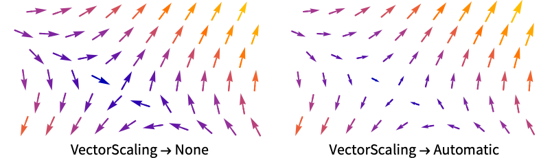
Axes True whether to draw axes BoundaryStyle Automatic how to style surface boundaries BoxRatios {1,1,1} ratio of height to width ClippingStyle Automatic how to display arrows outside the vector range DataRange Automatic the range of x, y, and z values to assume for data Method Automatic methods to use for the plot PerformanceGoal $PerformanceGoal aspects of performance to try to optimize PlotPoints Automatic approximate number of samples for the slice surfaces surfi in each direction PlotRange {Full,Full,Full} range of x, y, z values to include PlotRangePadding Automatic how much to pad the range of values PlotStyle Automatic style directives for each slice surface PlotTheme $PlotTheme overall theme for the plot RegionBoundaryStyle None how to style plot region boundaries RegionFunction (True&) determine what region to include ScalingFunctions None how to scale axes TargetUnits Automatic desired units to use VectorAspectRatio Automatic width-to-length ratio for arrows VectorColorFunction Automatic how to color vectors VectorColorFunctionScaling True whether to scale the argument to VectorColorFunction VectorMarkers Automatic the shape of the arrows VectorPoints Automatic the number or placement of vectors to plot VectorRange Automatic range of vector lengths to show VectorScaling None how to scale the sizes of arrows VectorSizes Automatic sizes of displayed arrows VectorStyle Automatic how to draw vectors - VectorScaling scales the magnitudes of the vectors into the range of arrow sizes smin to smax given by VectorSizes.
- VectorScaling->Automatic will scale the arrow lengths depending on the vector magnitudes:
- RegionFunction is supplied with x, y, z, vx, vy, vz, Norm[{vx,vy,vz}].
- VectorColorFunction is by default supplied with scaled x, y, z, vx, vy, vz, Norm[{vx,vy,vz}].
- For an array of dimension {r,s,t,3}, the setting DataRangeAutomatic is equivalent to DataRange{{1,r},{1,s},{1,t}}.
- Slice surfaces can be styled using a Style wrapper and PlotStyle option with the Style wrapper taking precedence over PlotStyle. None can be used to indicate that no slice surface should be shown.
- Possible settings for ScalingFunctions include:
-
{sx,sy,sz} scale x, y and z axes - Common built-in scaling functions s include:
-
"Log" 
log scale with automatic tick labeling "Log10" 
base-10 log scale with powers of 10 for ticks "SignedLog" 
log-like scale that includes 0 and negative numbers "Reverse" 
reverse the coordinate direction
List of all options
Examples
open all close allBasic Examples (2)
Plot a vector field over a surface:
data = Table[{y, -x, z}, {z, -3, 3}, {y, -2, 2}, {x, -2, 2}];ListSliceVectorPlot3D[data, "CenterPlanes"]data = Table[{y, -x, z}, {z, -2, 2}, {y, -2, 2}, {x, -2, 2}];ListSliceVectorPlot3D[data, ImplicitRegion[x ^ 2 - y ^ 2 - z == 0, {x, y, z}], DataRange -> {{-2, 2}, {-2, 2}, {-2, 2}}]Scope (21)
Surfaces (9)
Generate a plot over standard slice surfaces:
data = Table[{y, -x, z}, {z, -2, 2}, {y, -2, 2}, {x, -2, 2}];Table[ListSliceVectorPlot3D[data, sl, PlotLabel -> sl], {sl, {"CenterPlanes", "BackPlanes", "DiagonalStackedPlanes"}}]Standard axis-aligned stacked slice surfaces:
data = Table[{y, -x, z}, {z, -2, 2}, {y, -2, 2}, {x, -2, 2}];Table[ListSliceVectorPlot3D[data, sl, PlotLabel -> sl], {sl, {"XStackedPlanes", "YStackedPlanes", "ZStackedPlanes"}}]data = Table[{y, -x, z}, {z, -2, 2}, {y, -2, 2}, {x, -2, 2}];Table[ListSliceVectorPlot3D[data, sl, PlotLabel -> sl], {sl, {"CenterSphere", "CenterCutSphere", "CenterCutBox"}}]data = Table[{y, -x, z}, {z, -2, 2}, {y, -2, 2}, {x, -2, 2}];ListSliceVectorPlot3D[data, InfinitePlane[{{1, 0, 0}, {1, 1, 1}, {0, 0, 1}}], DataRange -> {{-2, 2}, {-2, 2}, {-2, 2}}]A volume slice region is equivalent to plotting over RegionBoundary[reg]:
data = Table[{y, -x, z}, {z, -1, 1}, {y, -1, 1}, {x, -1, 1}];ListSliceVectorPlot3D[data, Cylinder[], DataRange -> {{-1, 1}, {-1, 1}, {-1, 1}}]data = Table[{y, -x, z}, {z, -1, 1}, {y, -1, 1}, {x, -1, 1}];ListSliceVectorPlot3D[data, ImplicitRegion[ x ^ 3 + y ^ 2 - z ^ 2 == 0, {x, y, z}], DataRange -> {{-1, 1}, {-1, 1}, {-1, 1}}]Plot over multiple slice surfaces:
data = Table[{y, -x, z}, {z, -2, 2}, {y, -2, 2}, {x, -2, 2}];ListSliceVectorPlot3D[data, {Cylinder[], "BackPlanes"}, DataRange -> {{-2, 2}, {-2, 2}, {-2, 2}}]Specify the number of stacked planes:
data = Table[{y, -x, z}, {z, -2, 2}, {y, -2, 2}, {x, -2, 2}];ListSliceVectorPlot3D[data, {"XStackedPlanes", 7}]Specify the cutting angle for a center-cut sphere slice:
data = Table[{y, -x, z}, {z, -2, 2}, {y, -2, 2}, {x, -2, 2}];ListSliceVectorPlot3D[data, {"CenterCutSphere", 2Pi / 3}]Data (4)
For regular data consisting of ![]() vectors, the
vectors, the ![]() ,
, ![]() , and
, and ![]() data reflects its positions in the array:
data reflects its positions in the array:
data = Table[{y, -x, z}, {z, -2, 2}, {y, -2, 2}, {x, -2, 2}];ListSliceVectorPlot3D[data, "CenterPlanes"]Provide explicit ![]() ,
, ![]() , and
, and ![]() data ranges by using DataRange:
data ranges by using DataRange:
ListSliceVectorPlot3D[data, "CenterPlanes", DataRange -> {{-2, 2}, {-2, 2}, {-2, 2}}]Use VectorPoints to specify the number of arrows:
data = Table[{x, y, z}, {z, -1, 1}, {y, -1, 1}, {x, -1, 1}];ListSliceVectorPlot3D[data, "BackPlanes", VectorPoints -> 5]Plot a vector field given by QuantityArray:
data = QuantityArray[Table[{y, -x, z}, {z, -2, 2}, {y, -2, 2}, {x, -2, 2}], "kg/m^3"];ListSliceVectorPlot3D[data, "BackPlanes", AxesLabel -> Automatic, TargetUnits -> {"Feet", "Feet", "Feet", "g/ft^3"}]Use RegionFunction to expose obscured slices:
data = Table[{y, -x, z}, {z, -2, 2}, {y, -2, 2}, {x, -2, 2}];ListSliceVectorPlot3D[data, "ZStackedPlanes", RegionFunction -> Function[{x, y, z}, x < 0 || y > 0], DataRange -> {{-2, 2}, {-2, 2}, {-2, 2}}]Presentation (8)
Use PlotTheme to immediately get overall styling:
data = Table[{y, -x, z}, {z, -2, 2}, {y, -2, 2}, {x, -2, 2}];Table[ListSliceVectorPlot3D[data, "CenterPlanes", PlotLabel -> t, PlotTheme -> t, ImageSize -> 130], {t, {"Minimal", "Scientific", "Marketing"}}]Control the display of axes with Axes:
data = Table[{y, -x, z}, {z, -2, 2}, {y, -2, 2}, {x, -2, 2}];Table[ListSliceVectorPlot3D[data, "CenterPlanes", PlotLabel -> a, Axes -> a], {a, {True, False, {True, False, True}}}]Label axes using AxesLabel and the whole plot using PlotLabel:
data = Table[{y, -x, z}, {z, -2, 2}, {y, -2, 2}, {x, -2, 2}];ListSliceVectorPlot3D[data, "CenterPlanes", Ticks -> None, AxesLabel -> {x, y, z}, PlotLabel -> {y, -x, z}]Color the vectors by their magnitude with VectorColorFunction:
data = Table[{y, -x, z}, {z, -2, 2}, {y, -2, 2}, {x, -2, 2}];Table[ListSliceVectorPlot3D[data, "BackPlanes", PlotLabel -> c, VectorColorFunction -> c], {c, {Hue, "RedBlueTones"}}]Use VectorStyle to control the shape of the vectors:
data = Table[{y, -x, z}, {z, -1, 1}, {y, -1, 1}, {x, -1, 1}];Table[ListSliceVectorPlot3D[data, "CenterSphere", PlotLabel -> s, VectorMarkers -> s, VectorPoints -> 5, ImageSize -> Small], {s, {"Arrow3D", "Segment"}}]Scale to reflect vector magnitudes:
data = Table[{x, y, z}, {z, -1, 1}, {y, -1, 1}, {x, -1, 1}];ListSliceVectorPlot3D[data, "CenterPlanes", VectorScaling -> Automatic]Style the slice surface boundaries with BoundaryStyle:
data = Table[{y, -x, z}, {z, -2, 2}, {y, -2, 2}, {x, -2, 2}];ListSliceVectorPlot3D[data, "CenterPlanes", BoundaryStyle -> Red]TargetUnits specifies which units to use in the visualization:
data = QuantityArray[Table[{y, -x, z}, {z, -2, 2}, {y, -2, 2}, {x, -2, 2}], "kg/m^3"];ListSliceVectorPlot3D[data, "BackPlanes", AxesLabel -> Automatic, TargetUnits -> {"Feet", "Feet", "Feet", "g/ft^3"}]Options (48)
BoundaryStyle (1)
BoxRatios (3)
By default, the edges of the bounding box have the same length:
data = Table[{y, -x, z}, {z, -2, 2}, {y, -2, 2}, {x, -3, 3}];ListSliceVectorPlot3D[data, "CenterSphere"]Use BoxRatios-> Automatic to show the natural scale of the 3D coordinate values:
data = Table[{y, -x, z}, {z, -3, 3}, {y, -2, 2}, {x, -2, 2}];ListSliceVectorPlot3D[data, "CenterSphere", BoxRatios -> Automatic]Use custom length ratios for each side of the bounding box:
data = Table[{y, -x, z}, {z, -3, 3}, {y, -2, 2}, {x, -2, 2}];ListSliceVectorPlot3D[data, "CenterSphere", BoxRatios -> {2, 1, 1}]ClippingStyle (4)
By default, clipped vectors are given a constant color that is consistent with the minimum or maximum vector lengths given by VectorRange:
data = Table[{z^2, y^2, x^2}, {z, -5, 5}, {y, -5, 5}, {x, -5, 5}];ListSliceVectorPlot3D[data, "CenterPlanes", VectorRange -> {5, 15}]data = Table[{z^2, y^2, x^2}, {z, -5, 5}, {y, -5, 5}, {x, -5, 5}];ListSliceVectorPlot3D[data, "CenterPlanes", VectorRange -> {5, 15}, ClippingStyle -> None]data = Table[{z^2, y^2, x^2}, {z, -5, 5}, {y, -5, 5}, {x, -5, 5}];ListSliceVectorPlot3D[data, "CenterPlanes", VectorRange -> {5, 15}, ClippingStyle -> Black]Style the short and long clipped vectors differently:
data = Table[{z^2, y^2, x^2}, {z, -5, 5}, {y, -5, 5}, {x, -5, 5}];ListSliceVectorPlot3D[data, "CenterPlanes", VectorRange -> {5, 15}, ClippingStyle -> {White, Black}]DataRange (2)
By default, the data range is taken to be the dimension of the array:
data = Table[{x, y, z}, {z, -2, 2}, {y, -2, 2}, {x, -2, 2}];ListSliceVectorPlot3D[data, "CenterPlanes"]Explicitly specify the data range:
data = Table[{x, y, z}, {z, -2, 2}, {y, -2, 2}, {x, -2, 2}];ListSliceVectorPlot3D[data, "CenterPlanes", DataRange -> {{-2, 2}, {-2, 2}, {-2, 2}}]PerformanceGoal (2)
Generate a higher-quality plot:
data = Table[{y, -x, z}, {z, -2, 2}, {y, -2, 2}, {x, -2, 2}];Timing[ListSliceVectorPlot3D[data, "CenterPlanes", PerformanceGoal -> "Quality"]]Emphasize performance, possibly at the cost of quality:
data = Table[{y, -x, z}, {z, -2, 2}, {y, -2, 2}, {x, -2, 2}];Timing[ListSliceVectorPlot3D[data, "CenterPlanes", PerformanceGoal -> "Speed"]]PlotLegends (1)
PlotRange (2)
Show All vectors by default:
data = Table[{y, -x, z}, {z, -2, 2}, {y, -2, 2}, {x, -2, 2}];ListSliceVectorPlot3D[data, "CenterSphere"]data = Table[{y, -x, z}, {z, -2, 2}, {y, -2, 2}, {x, -2, 2}];ListSliceVectorPlot3D[data, "CenterSphere", PlotRange -> {All, All, {-2, 0}}, DataRange -> {{-2, 2}, {-2, 2}, {-2, 2}}, BoxRatios -> Automatic]PlotRangePadding (5)
Padding is computed automatically by default:
data = Table[{y, -x, z}, {z, -2, 2}, {y, -2, 2}, {x, -2, 2}];ListSliceVectorPlot3D[data, "BackPlanes"]Specify no padding for all ![]() ,
, ![]() , and
, and ![]() ranges:
ranges:
data = Table[{y, -x, z}, {z, -2, 2}, {y, -2, 2}, {x, -2, 2}];ListSliceVectorPlot3D[data, "BackPlanes", PlotRangePadding -> None]Specify an explicit padding for all ![]() ,
, ![]() , and
, and ![]() ranges:
ranges:
data = Table[{y, -x, z}, {z, -2, 2}, {y, -2, 2}, {x, -2, 2}];ListSliceVectorPlot3D[data, "BackPlanes", PlotRangePadding -> 1]Add 10% padding to all ![]() ,
, ![]() , and
, and ![]() ranges:
ranges:
data = Table[{y, -x, z}, {z, -2, 2}, {y, -2, 2}, {x, -2, 2}];ListSliceVectorPlot3D[data, "BackPlanes", PlotRangePadding -> Scaled[0.1]]Specify padding for ![]() and
and ![]() ranges:
ranges:
data = Table[{y, -x, z}, {z, -2, 2}, {y, -2, 2}, {x, -2, 2}];ListSliceVectorPlot3D[data, "BackPlanes", PlotRangePadding -> {1, 0.5}]PlotTheme (3)
data = Table[{y, -x, z}, {z, -2, 2}, {y, -2, 2}, {x, -2, 2}];ListSliceVectorPlot3D[data, "CenterPlanes", PlotTheme -> "Marketing"]Regular options override PlotTheme settings, in this case turning off FaceGrids:
data = Table[{y, -x, z}, {z, -2, 2}, {y, -2, 2}, {x, -2, 2}];ListSliceVectorPlot3D[data, "CenterPlanes", PlotTheme -> "Marketing", FaceGrids -> None]Compare different plot themes:
data = Table[{y, -x, z}, {z, -2, 2}, {y, -2, 2}, {x, -2, 2}];Table[ListSliceVectorPlot3D[data, "CenterPlanes", PlotLabel -> t, PlotTheme -> t, ImageSize -> 130], {t, {"Scientific", "Monochrome", "Minimal", "Web", "Working", "Classic", "Business", "Marketing", "Detailed"}}]RegionFunction (2)
Use RegionFunction to specify what regions of the slice surfaces to include:
data = Table[{x, y, z}, {z, -2, 2}, {y, -2, 2}, {x, -2, 2}];ListSliceVectorPlot3D[data, "CenterSphere", RegionFunction -> ((#1 #2 #3 > 0)&), DataRange -> {{-2, 2}, {-2, 2}, {-2, 2}}]Plot vectors only over regions where the field magnitude is above a given threshold:
data = Table[{x, y, z}, {z, -2, 2}, {y, -2, 2}, {x, -2, 2}];ListSliceVectorPlot3D[data, "BackPlanes", RegionFunction -> ((2.5 < #7)&), DataRange -> {{-2, 2}, {-2, 2}, {-2, 2}}]VectorColorFunction (5)
By default, vectors are colored according to their norm:
data = Table[{y, -x, z}, {z, -2, 2}, {y, -2, 2}, {x, -2, 2}];ListSliceVectorPlot3D[data, "BackPlanes"]data = Table[{y, -x, z}, {z, -2, 2}, {y, -2, 2}, {x, -2, 2}];ListSliceVectorPlot3D[data, "BackPlanes", VectorColorFunction -> Hue]Use any named color gradient from ColorData:
data = Table[{y, -x, z}, {z, -2, 2}, {y, -2, 2}, {x, -2, 2}];ListSliceVectorPlot3D[data, "BackPlanes", VectorColorFunction -> "TemperatureMap"]Color the vectors according to their ![]() value:
value:
data = Table[{y, -x, z}, {z, -2, 2}, {y, -2, 2}, {x, -2, 2}];ListSliceVectorPlot3D[data, "BackPlanes", VectorColorFunction -> Function[{x, y, z, vx, vy, vz, n}, ColorData["ThermometerColors"][x]]]Use VectorColorFunctionScalingFalse to get unscaled values:
data = Table[{y, -x, z}, {z, -2, 2}, {y, -2, 2}, {x, -2, 2}];ListSliceVectorPlot3D[data, "CenterPlanes", VectorColorFunction -> (If[#7 > 1.6, Red, Blue]&), VectorColorFunctionScaling -> False]VectorColorFunctionScaling (3)
By default, scaled values are used:
data = Table[{x, y, z}, {z, -1, 1}, {y, -1, 1}, {x, -1, 1}];ListSliceVectorPlot3D[data, "CenterPlanes"]Use VectorColorFunctionScaling->False to get unscaled values:
data = Table[{x, y, z}, {z, -1, 1, 0.2}, {y, -1, 1, 0.2}, {x, -1, 1, 0.2}];ListSliceVectorPlot3D[data, "CenterPlanes", VectorColorFunction -> (If[#7 > 0.8, Red, Blue]&), VectorColorFunctionScaling -> False]Explicitly specify the scaling for each color function argument:
data = Table[{x, y, z}, {z, -2, 2}, {y, -2, 2}, {x, -2, 2}];ListSliceVectorPlot3D[data, "CenterPlanes", VectorColorFunction -> (If[Abs[#1] < 1, Black, Hue[#7]]&), VectorColorFunctionScaling -> {False, True}, DataRange -> {{-2, 2}, {-2, 2}, {-2, 2}}]VectorMarkers (2)
The default vector marker is "Arrow3D":
data = Table[{y, -x, 0}, {z, -1, 1, 0.5}, {y, -1, 1, 0.5}, {x, -1, 1, 0.5}];ListSliceVectorPlot3D[data, "CenterSphere", VectorMarkers -> "Arrow3D"]data = Table[{y, -x, 0}, {z, -1, 1, 0.5}, {y, -1, 1, 0.5}, {x, -1, 1, 0.5}];Table[ListSliceVectorPlot3D[data, "CenterSphere", VectorMarkers -> m, PlotLabel -> m], {m, {"Tube", "Segment", "Arrow"}}]VectorPoints (3)
Use automatically determined vector points:
data = Table[{x, y, z}, {z, -1, 1}, {y, -1, 1}, {x, -1, 1}];ListSliceVectorPlot3D[data, "BackPlanes", VectorPoints -> Automatic]Use symbolic names to specify the set of field vectors:
data = Table[{x, y, z}, {z, -1, 1}, {y, -1, 1}, {x, -1, 1}];Table[ListSliceVectorPlot3D[data, "BackPlanes", PlotLabel -> k, VectorPoints -> k, PlotTheme -> "Minimal"], {k, {Fine, Coarse}}]Create a regular grid of field vectors with the same number of arrows for ![]() ,
, ![]() , and
, and ![]() :
:
data = Table[{x, y, z}, {z, -1, 1}, {y, -1, 1}, {x, -1, 1}];ListSliceVectorPlot3D[data, "BackPlanes", VectorPoints -> 5]VectorRange (3)
Specify the range of vector norms that are displayed with varying color:
data = Table[{y z, -x z, x y}, {z, -3, 3}, {y, -3, 3}, {x, -3, 3}];ListSliceVectorPlot3D[data, "CenterPlanes", VectorRange -> {1, 5}]Combine with ClippingStyle to remove the clipped vectors:
data = Table[{y z, -x z, x y}, {z, -3, 3}, {y, -3, 3}, {x, -3, 3}];ListSliceVectorPlot3D[data, "CenterPlanes", VectorRange -> {1, 5}, ClippingStyle -> None]Or specify a different style for clipped vectors:
data = Table[{y z, -x z, x y}, {z, -3, 3}, {y, -3, 3}, {x, -3, 3}];ListSliceVectorPlot3D[data, "CenterPlanes", VectorRange -> {1, 5}, ClippingStyle -> Black]VectorScaling (3)
By default, arrows are displayed with a constant length:
data = Table[{x, y, z}, {z, -2, 2}, {y, -2, 2}, {x, -2, 2}];ListSliceVectorPlot3D[data, "CenterPlanes"]Use Automatic to scale arrows proportionally to the corresponding vector norm:
data = Table[{x, y, z}, {z, -2, 2}, {y, -2, 2}, {x, -2, 2}];ListSliceVectorPlot3D[data, "CenterPlanes", VectorScaling -> Automatic]Use VectorSizes to specify the range of relative lengths of the arrows:
data = Table[{x, y, z}, {z, -2, 2}, {y, -2, 2}, {x, -2, 2}];ListSliceVectorPlot3D[data, "CenterPlanes", VectorScaling -> Automatic, VectorSizes -> {0.5, 1}]VectorSizes (2)
Make the vectors half of the default size:
data = Table[{x, y, z}, {z, -2, 2}, {y, -2, 2}, {x, -2, 2}];ListSliceVectorPlot3D[data, "CenterCutSphere", VectorSizes -> {0, 0.5}]With VectorScaling, VectorSizes controls the range of the lengths of the arrows relative to the default size:
data = Table[{x, y, z}, {z, -2, 2}, {y, -2, 2}, {x, -2, 2}];ListSliceVectorPlot3D[data, "CenterCutSphere", VectorScaling -> Automatic, VectorSizes -> {0.5, 0.7}]VectorStyle (1)
VectorColorFunction has precedence over VectorStyle:
data = Table[{y, -x, z}, {z, -1, 1}, {y, -1, 1}, {x, -1, 1}];ListSliceVectorPlot3D[data, "CenterSphere", VectorStyle -> Red]ListSliceVectorPlot3D[data, "CenterSphere", VectorStyle -> Red, VectorColorFunction -> None]TargetUnits (1)
Applications (7)
Basic Vector Fields (3)
Constant vector fields from data:
data = Table[{1, 0, 0}, {z, -1, 1}, {y, -1, 1}, {x, -1, 1}];ListSliceVectorPlot3D[data, "CenterPlanes", VectorPoints -> 6]{ListSliceVectorPlot3D[Table[{0, 1, 0}, {z, -1, 1}, {y, -1, 1}, {x, -1, 1}], "CenterPlanes", VectorPoints -> 6], ListSliceVectorPlot3D[Table[{0, 0, 1}, {z, -1, 1}, {y, -1, 1}, {x, -1, 1}], "CenterPlanes", VectorPoints -> 6]}data = Table[{y, -x, 0}, {z, -1, 1}, {y, -1, 1}, {x, -1, 1}];ListSliceVectorPlot3D[data, Cylinder[], DataRange -> {{-1, 1}, {-1, 1}, {-1, 1}}]ListSliceVectorPlot3D[Table[{x, y, z}, {z, -1, 1}, {y, -1, 1}, {x, -1, 1}], "CenterCutSphere"]ListSliceVectorPlot3D[Table[-{x, y, z}, {z, -1, 1}, {y, -1, 1}, {x, -1, 1}], "CenterCutSphere"]Image Processing (1)
Visualize the gradient vectors of a 3D image:
img = [image];Compute the vector orientations:
dirs = ImageData[GradientOrientationFilter[img, 5]];
magnitudes = ImageData[GradientFilter[img, 5]];vectors = MapThread[#1{Cos[#2[[1]]], Sin[#2[[1]]]Cos[#2[[2]]], Sin[#2[[1]]]Sin[#2[[2]]]}&, {magnitudes, dirs}, 3];Show the vectors with the image:
vp = ListSliceVectorPlot3D[vectors, {"XStackedPlanes", 4}]Show[img, vp]Fluid Dynamics (2)
Visualize Hill's spherical vortex, with vortex radius ![]() and velocity
and velocity ![]() :
:
{R, U} = {1, 2};{u, v, w} = U{(x z/R^2), (y z/R^2), 1 - ((z/R))^2 - 2((x^2 + y^2/R^2))};data = Table[{u, v, w}, {z, -1.5, 1.5, 0.1}, {y, -1.5, 1.5, 0.1}, {x, -1.5, 1.5, 0.1}];Visualize the vortex by coloring based on the flow speed:
ListSliceVectorPlot3D[data, {"CenterCutSphere", 2Pi / 3}, VectorPoints -> 20, VectorColorFunction -> (If[#7 < 0.3, Red, Gray]&)]Visualize the divergence-free field of a scalar function ![]() :
:
ϕ = (6/E^x^2 + y^2 + z^2) + Sqrt[1 + 3((x - 1)^2 + (y - 1)^2 + (z - 1)^2)];v1 = {-Laplacian[ϕ, {x, y, z}] + D[ϕ, {x, 2}], D[ϕ, x, y], D[ϕ, x, z]};
v2 = {D[ϕ, x, y], -Laplacian[ϕ, {x, y, z}] + D[ϕ, {y, 2}], D[ϕ, y, z]};
v3 = {D[ϕ, x, z], D[ϕ, y, z], -Laplacian[ϕ, {x, y, z}] + D[ϕ, {z, 2}]};{data1, data2, data3} = Table[vectorField, {vectorField, {v1, v2, v3}}, {z, -2, 2, 0.11}, {y, -2, 2, 0.11}, {x, -2, 2, 0.11}];Visualize the vortices formed by these fields:
ListSliceVectorPlot3D[data1, {{"YStackedPlanes", 1}, {"ZStackedPlanes", 1}}, VectorPoints -> 12, PlotTheme -> "Minimal", VectorScaling -> Automatic, VectorAspectRatio -> 0.2]{ListSliceVectorPlot3D[data2, {{"XStackedPlanes", 1}, {"ZStackedPlanes", 1}}, VectorPoints -> 12, PlotTheme -> "Minimal", VectorScaling -> Automatic, VectorAspectRatio -> 0.2], ListSliceVectorPlot3D[data3, {{"XStackedPlanes", 1}, {"YStackedPlanes", 1}}, VectorPoints -> 12, PlotTheme -> "Minimal", VectorScaling -> Automatic, VectorAspectRatio -> 0.2]}Gradient Fields (1)
Observe the gradient field superimposed on a density plot of a function:
f[x_, y_, z_] := (x - 1)^2 + y^2 + z^2data = Table[f[x, y, z], {z, -2, 2}, {y, -2, 2}, {x, -2, 2}];gradientdata = Table[Evaluate[Grad[f[x, y, z], {x, y, z}]], {z, -2, 2}, {y, -2, 2}, {x, -2, 2}];Show[ListSliceDensityPlot3D[data, "CenterCutSphere", ColorFunction -> GrayLevel, DataRange -> {{-2, 2}, {-2, 2}, {-2, 2}}],
ListSliceVectorPlot3D[gradientdata, "CenterCutSphere", VectorColorFunction -> "CMYKColors", DataRange -> {{-2, 2}, {-2, 2}, {-2, 2}}, PlotStyle -> None]]Properties & Relations (8)
Use ListVectorPlot3D for a full volume visualization of the vector field:
data = Table[{y, -x, z}, {z, -2, 2}, {y, -2, 2}, {x, -2, 2}];{ListVectorPlot3D[data], ListSliceVectorPlot3D[data, "CenterPlanes"]}Use SliceVectorPlot3D for functions:
data = Table[{y, -x, z}, {z, -2, 2}, {y, -2, 2}, {x, -2, 2}];{SliceVectorPlot3D[{y, -x, z}, "CenterSphere", {x, -2, 2}, {y, -2, 2}, {z, -2, 2}], ListSliceVectorPlot3D[data, "CenterSphere"]}Use ListVectorPlot for vector plots in 2D:
data2D = Table[{y, -x}, {x, -3, 3}, {y, -3, 3}];data3D = Table[{y, -x, 0}, {z, -3, 3}, {y, -3, 3}, {x, -3, 3}];{ListVectorPlot[data2D], ListSliceVectorPlot3D[data3D, "BackPlanes"]}Use ListVectorDisplacementPlot or ListVectorDisplacementPlot3D to visualize displacement fields in 2D or 3D:
data2D = Table[{{x, y}, {y, -x}}, {x, -3, 3}, {y, -3, 3}];data3D = Table[{{x, y, z}, {y, -x, 0}}, {z, -3, 3}, {y, -3, 3}, {x, -3, 3}];{ListVectorDisplacementPlot[data2D, VectorPoints -> Automatic],
ListVectorDisplacementPlot3D[data3D, VectorPoints -> "Boundary"]}Use ListStreamPlot or ListLineIntegralConvolutionPlot for vector fields in 2D:
data = Table[{y, -x}, {x, -3, 3}, {y, -3, 3}];{ListStreamPlot[data],
ListLineIntegralConvolutionPlot[data]}Use ListVectorDensityPlot or ListStreamDensityPlot to include a scalar field in 2D:
data = Table[{y, -x}, {x, -3, 3}, {y, -3, 3}];{ListVectorDensityPlot[data], ListStreamDensityPlot[data]}Use ListStreamPlot3D to visualize 3D vector field data as streamlines:
ListStreamPlot3D[Table[{z, -x, y}, {x, -1, 1, .1}, {y, -1, 1, .1}, {z, -1, 1, .1}]]Use GeoVectorPlot to plot vectors on a map:
GeoVectorPlot[GeoVector[GeoPosition[{{-54.79801473961214, -111.85053058521567},
    {-65.56940402358214, 162.89657500795147}, {-81.67990688759895, -93.36222177594851},
    {7.785750774919734, 95.44840765141487}, {-6.86571958448036, -40.946398330539864},
    { ... 904, "AngularDegrees"]},
   {0.9366099079317551, Quantity[357.70482317743733, "AngularDegrees"]},
   {0.8256817194791912, Quantity[242.07227508889662, "AngularDegrees"]},
   {0.2661401145642981, Quantity[152.90003252279325, "AngularDegrees"]}}]]
Use GeoStreamPlot to plot streams instead of vectors:
GeoStreamPlot[GeoVector[GeoPosition[{{-54.79801473961214, -111.85053058521567},
    {-65.56940402358214, 162.89657500795147}, {-81.67990688759895, -93.36222177594851},
    {7.785750774919734, 95.44840765141487}, {-6.86571958448036, -40.946398330539864},
    { ... 904, "AngularDegrees"]},
   {0.9366099079317551, Quantity[357.70482317743733, "AngularDegrees"]},
   {0.8256817194791912, Quantity[242.07227508889662, "AngularDegrees"]},
{0.2661401145642981, Quantity[152.90003252279325, "AngularDegrees"]}}]]Text
Wolfram Research (2015), ListSliceVectorPlot3D, Wolfram Language function, https://reference.wolfram.com/language/ref/ListSliceVectorPlot3D.html (updated 2022).
CMS
Wolfram Language. 2015. "ListSliceVectorPlot3D." Wolfram Language & System Documentation Center. Wolfram Research. Last Modified 2022. https://reference.wolfram.com/language/ref/ListSliceVectorPlot3D.html.
APA
Wolfram Language. (2015). ListSliceVectorPlot3D. Wolfram Language & System Documentation Center. Retrieved from https://reference.wolfram.com/language/ref/ListSliceVectorPlot3D.html