


ReImPlot
ReImPlot[f,{x,xmin,xmax}]
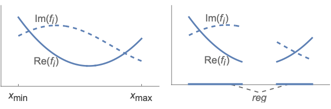
generates a plot of Re[f] and Im[f] as functions of x∈ from xmin to xmax.
ReImPlot[{f1,f2,…},{x,xmin,xmax}]
plots several functions.
ReImPlot[{…,w[fi],…},…]
plots fi with features defined by the symbolic wrapper w.
ReImPlot[…,{x}∈reg]
takes the variable x to be in the geometric region reg.
Details and Options
- ReImPlot evaluates f at different values of x to create smooth curves of the form {x,Re[f[x]]} and {x,Im[f[x]]}.
- Gaps are left at any x where the fi evaluate to non-numeric values.
- The region reg can be any RegionQ object in 1D.
- ReImPlot treats the variable x as local, effectively using Block.
- ReImPlot has attribute HoldAll and evaluates f only after assigning specific numerical values to x.
- In some cases, it may be more efficient to use Evaluate to evaluate f symbolically before specific numerical values are assigned to x.
- Wrappers apply to both Re[f] and Im[f].
- The following wrappers w can be used for the fi:
-
Annotation[fi,label] provide an annotation for the fi Button[fi,action] evaluate action when the curve for fi is clicked Callout[fi,label] label the function with a callout Callout[fi,label,pos] place the callout at relative position pos EventHandler[fi,events] define a general event handler for fi Highlighted[fi,effect] dynamically highlight fi with an effect Highlighted[fi,Placed[effect,pos]] statically highlight fi with an effect at position pos Hyperlink[fi,uri] make the function a hyperlink Labeled[fi,label] label the function Labeled[fi,label,pos] place the label at relative position pos Legended[fi,label] identify the function in a legend PopupWindow[fi,cont] attach a popup window to the function StatusArea[fi,label] display in the status area on mouseover Style[fi,styles] show the function using the specified styles Tooltip[fi,label] attach a tooltip to the function Tooltip[fi] use functions as tooltips - Wrappers w can be applied at multiple levels:
-
w[fi] wrap the fi w[{f1,…}] wrap a collection of fi w1[w2[…]] use nested wrappers - Callout, Labeled and Placed can use the following positions pos:
-
Automatic automatically placed labels Above, Below, Before, After positions around the curve x near the curve at a position x Scaled[s] scaled position s along the curve {s,Above},{s,Below},… relative position at position s along the curve {pos,epos} epos in label placed at relative position pos of the curve - ReImPlot has the same options as Plot, with the following additions and changes: [List of all options]
-
ReImLabels Automatic how to annotate the real and imaginary components ReImStyle Automatic how to style the real and imaginary components PlotStyle Automatic how to style individual functions fi - Possible settings for ClippingStyle are:
-
Automatic use a dotted line for the clipped portion 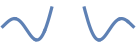
None omit the clipped portion of the curve 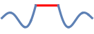
style use style for the clipped portion - With the default settings Exclusions->Automatic and ExclusionsStyle->None, Plot breaks curves at discontinuities and singularities it detects. Exclusions->None joins across discontinuities and singularities.
- Exclusions->{x1,x2,…} is equivalent to Exclusions->{x==x1,x==x2,…}.
- Possible settings for PlotLegends are:
-
None do not include legends "Expressions" use a legend for the fi "ReIm" use a legend for the real and imaginary styles "ReImExpressions" use separate legends for the plot, real and imaginary styles Automatic use a legend for all style combinations {lbl1,lbl2,…} use lbli to legend fi Placed[leg,pos] specify placement pos of legend leg {leg1,leg2,…} include multiple legends - PlotStyle determines the style for each function, and ReImStyle determines the style for the real and imaginary components.
- Possible settings for ReImStyle include:
-
Automatic default styles {re,im} use re and im for the respective components {{re1,im1},{re2,im2},…} use different styles for different functions - ColorData["DefaultPlotColors"] gives the default sequence of colors used by PlotStyle.
- Possible highlighting effects for Highlighted and PlotHighlighting include:
-

style highlight the indicated curve 
"Ball" highlight and label the indicated point in a curve 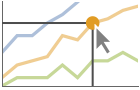
"Dropline" highlight and label the indicated point in a curve with droplines to the axes 
"XSlice" highlight and label all points along a vertical slice 
"YSlice" highlight and label all points along a horizontal slice 
Placed[effect,pos] statically highlight the given position pos - Highlight position specifications pos include:
-
x, {x} effect at {x,y} with y chosen automatically {x,y} effect at {x,y} {pos1,pos2,…} multiple positions posi - ReImPlot initially evaluates f at a number of equally spaced sample points specified by PlotPoints. Then it uses an adaptive algorithm to choose additional sample points, subdividing a given interval at most MaxRecursion times.
- Since only a finite number of sample points are used, it is possible for ReImPlot to miss features of f. Increasing the settings for PlotPoints and MaxRecursion will often catch such features.
- Themes that affect curves include:
-

"ThinLines" thin plot lines 
"MediumLines" medium plot lines 
"ThickLines" thick plot lines - The arguments supplied to functions in MeshFunctions and RegionFunction are x, y. Functions in ColorFunction are by default supplied with scaled versions of these arguments.
- ScalingFunctions->"scale" scales the
 coordinate; ScalingFunctions{"scalex","scaley"} scales both the
  and
and  coordinates.

List of all options
Examples
open all close allBasic Examples (3)
Plot the real and imaginary parts of a complex-valued function of a real variable:
ReImPlot[Sqrt[(x^2 - 1)(x^2 - 4)], {x, -3, 3}]ReImPlot[{ArcSin[x], ArcCos[x]}, {x, -4, 4}]ReImPlot[{ArcSin[x], ArcCos[x]}, {x, -4, 4}, PlotLabels -> "Expressions"]Scope (23)
Sampling (9)
More points are sampled where the function changes quickly:
ReImPlot[Exp[30I Sin[x]], {x, 0, 10}]The plot range is selected automatically:
ReImPlot[Exp[(1 / 2 + I) t], {t, -2π, 3π}]Use PlotRange to focus in on areas of interest:
ReImPlot[Exp[(1 / 2 + I) t], {t, -2π, 3π}, PlotRange -> {-70, 70}]The curve is split when there are discontinuities in the function:
ReImPlot[Floor[Sqrt[x]], {x, -100, 100}]Use ExclusionsNone to draw connected curves:
ReImPlot[Floor[Sqrt[x]], {x, -100, 100}, Exclusions -> None]Use PlotPoints and MaxRecursion to control adaptive sampling:
Grid@Table[ReImPlot[Exp[I x], {x, 0, 15}, PlotPoints -> pp, MaxRecursion -> mr], {mr, {0, 1, 2}}, {pp, {5, 10}}]The domain can be specified by a region:
𝒟 = ImplicitRegion[-4 ≤ x ≤ -1∨1 ≤ x ≤ 4, {x}];ReImPlot[Exp[I x], {x}∈𝒟]Specify a domain using a MeshRegion:
𝒟 = MeshRegion[{{-2}, {-1}, {-1 / 2}, {1 / 2}, {1}, {2}}, Line[{{1, 2}, {3, 4}, {5, 6}}]];ReImPlot[Sin[x^2] - I, {x}∈𝒟]ReImPlot[Exp[-(1 / 2 + I) t], {t, 0, Infinity}, PlotRange -> All]Labeling and Legending (8)
There are two standard legends:
ReImPlot[{ArcCos[x], ArcSin[x]}, {x, -3, 3}, PlotLegends -> {"Expressions", "ReIm"}]ReImPlot[{ArcCos[x], ArcSin[x]}, {x, -3, 3}, PlotLegends -> "ReImExpressions"]Use legends with combined styles:
ReImPlot[{ArcCos[x], ArcSin[x]}, {x, -3, 3}, PlotLegends -> Automatic]Explicitly label the individual curves:
ReImPlot[{ArcCos[x], ArcSin[x]}, {x, -3, 3}, PlotLabels -> Automatic]Identify curves with wrappers:
ReImPlot[{Callout[ArcCos[x]], Tooltip[ArcSin[x], ArcSin[x]], Legended[ArcCos[x] + ArcSin[x], "sum"]}, {x, -3, 3}]Curves usually have interactive callouts showing the coordinates when you mouse over them:
ReImPlot[E^I / 2 x, {x, 0, 10}]Choose from multiple interactive highlighting effects:
{ReImPlot[{E^I / 2 x, E^I / 3 x}, {x, 0, 10}, PlotHighlighting -> "Dropline"], ReImPlot[{E^I / 2 x, E^I / 3 x}, {x, 0, 10}, PlotHighlighting -> "XSlice"]}Use Highlighted to emphasize specific points in a plot:
ReImPlot[Highlighted[E^I / 2 x, Placed["Ball", 5]], {x, 0, 10}]ReImPlot[Highlighted[E^I / 2 x, Placed["Ball", {{3}, {5}}]], {x, 0, 10}]Presentation (6)
Multiple pairs of curves are automatically colored to be distinct:
ReImPlot[{Sqrt[1 - x^2], -Sqrt[x^2 - 1]}, {x, -3, 3}]Provide explicit styling to different curves:
ReImPlot[{Sqrt[1 - x^2], -Sqrt[x^2 - 1]}, {x, -3, 3}, PlotStyle -> {Red, Blue}]ReImPlot[Sqrt[1 - x^2], {x, -3, 3}, AxesLabel -> {x, I y}, PlotLabel -> Sqrt[1 - x^2], PlotLegends -> "ReIm"]{ReImPlot[{Sqrt[1 - x^2], -Sqrt[x^2 - 1]}, {x, -3, 3}, Filling -> Axis], ReImPlot[{Sqrt[1 - x^2], -Sqrt[x^2 - 1]}, {x, -3, 3}, Filling -> {{2 -> {3}}, {1 -> {4}}}]}ReImPlot[{Sqrt[1 - x^2], -Sqrt[x^2 - 1]}, {x, -3, 3}, PlotTheme -> "Marketing"]Use ScalingFunctions to scale the axes:
ReImPlot[x + I Exp[x], {x, 0, 5}, ScalingFunctions -> "Log"]Options (65)
ClippingStyle (2)
ColorFunction (4)
Color by a scaled ![]() coordinate and scaled
coordinate and scaled ![]() coordinate, respectively:
coordinate, respectively:
{ReImPlot[{Sqrt[1 - x^2], -Sqrt[1 - x^2]}, {x, -3, 3}, ColorFunction -> Function[{x, y}, Hue[y]]],
ReImPlot[{Sqrt[1 - x^2], -Sqrt[1 - x^2]}, {x, -3, 3}, ColorFunction -> Function[{x, y}, Hue[x]]]}ReImPlot[{Sqrt[1 - x^2], -Sqrt[1 - x^2]}, {x, -3, 3}, ColorFunction -> "DarkRainbow"]ColorFunction has higher priority than PlotStyle:
ReImPlot[{Sqrt[1 - x^2], -Sqrt[1 - x^2]}, {x, -3, 3}, ColorFunction -> "DarkRainbow", PlotStyle -> Directive[Red, Thick]]ReImPlot[{Sqrt[1 - x^2], -Sqrt[1 - x^2]}, {x, -3, 3}, ColorFunction -> Function[{x, y}, If[Abs[y] ≤ 1, Red, Green]], ColorFunctionScaling -> False, PlotStyle -> Thick]ColorFunctionScaling (1)
Exclusions (2)
ExclusionStyle (1)
Filling (4)
Use symbolic or explicit values:
Table[ReImPlot[Exp[I x], {x, 0, 2Pi}, Filling -> f], {f, {Axis, Top, Bottom, .3}}]Fill between curve 1 and the ![]() axis:
axis:
ReImPlot[Exp[I x], {x, 0, 2Pi}, Filling -> {1 -> Axis}]ReImPlot[Exp[I x], {x, 0, 2Pi}, Filling -> {1 -> {2}}]Fill between the real and imaginary parts of each function:
ReImPlot[{Exp[I x], Exp[2I x]}, {x, 0, 2Pi}, Filling -> {{1 -> {3}}, {2 -> {4}}}]FillingStyle (3)
Table[ReImPlot[Exp[I x], {x, 0, 2Pi}, Filling -> Axis, FillingStyle -> c], {c, {Red, Green, Blue, Yellow}}]Fill with red below the ![]() axis and blue above:
axis and blue above:
ReImPlot[Exp[I x], {x, 0, 2Pi}, Filling -> Axis, FillingStyle -> {Red, Blue}]Use a variable filling style obtained from a ColorFunction:
ReImPlot[Exp[I x], {x, 0, 2Pi}, ColorFunction -> Function[{x, y}, Hue[x]], Filling -> {1 -> {2}}, FillingStyle -> Automatic]MaxRecursion (1)
Each level of MaxRecursion adaptively subdivides the initial mesh into a finer mesh:
Table[ReImPlot[Sin[1 / x] + 10 x I, {x, 0.001, .1}, MaxRecursion -> i, Mesh -> All, Ticks -> None], {i, {0, 3, 6}}]Mesh (3)
Show the initial and final sampling meshes:
{ReImPlot[Exp[I x], {x, 0, 2Pi}, Mesh -> Full, MeshStyle -> Red], ReImPlot[Exp[I x], {x, 0, 2Pi}, Mesh -> All, MeshStyle -> Red]}Use 10 mesh points evenly spaced in the ![]() direction:
direction:
ReImPlot[Exp[I x], {x, 0, 2Pi}, Mesh -> 10, MeshStyle -> Red]Use an explicit list of values for the mesh in the ![]() direction:
direction:
ReImPlot[Exp[I x], {x, 0, 2Pi}, Mesh -> {Range[0, 2Pi, Pi / 4]}, MeshStyle -> Red]MeshFunctions (2)
Use a mesh evenly spaced in the ![]() and
and ![]() directions:
directions:
Table[ReImPlot[Exp[I x], {x, 0, 2Pi}, MeshFunctions -> {f}, Mesh -> 15, MeshStyle -> Red], {f, {Function[{x, y, t, r}, x], Function[{x, y, t, r}, y]}}]Show seven mesh levels in the ![]() direction (red) and 15 in the
direction (red) and 15 in the ![]() direction (blue):
direction (blue):
ReImPlot[Exp[I x], {x, 0, 2Pi}, MeshFunctions -> {#1&, #2&}, Mesh -> {7, 15}, MeshStyle -> {Red, Blue}]MeshShading (3)
Alternate red and blue arcs in the ![]() direction:
direction:
ReImPlot[Exp[I x], {x, 0, 2Pi}, Mesh -> 7, MeshShading -> {Red, Blue}]MeshShading has higher priority than PlotStyle for styling:
ReImPlot[Exp[I x], {x, 0, 2Pi}, Mesh -> 7, MeshShading -> {Red, Blue}, PlotStyle -> Green]Use PlotStyle for some segments by setting MeshShading to Automatic:
ReImPlot[Exp[I x], {x, 0, 2Pi}, Mesh -> 7, MeshShading -> {Red, Automatic}, PlotStyle -> Green]MeshStyle (2)
Use a red mesh in the ![]() direction:
direction:
ReImPlot[Exp[I x], {x, 0, 2Pi}, Mesh -> 7, MeshStyle -> Red]Use a red mesh in the ![]() direction and a blue mesh in the
direction and a blue mesh in the ![]() direction:
direction:
ReImPlot[Exp[I x], {x, 0, 2Pi}, Mesh -> 7, MeshFunctions -> {#1&, #2&}, MeshStyle -> {Red, Blue}]PerformanceGoal (2)
PlotHighlighting (8)
Plots have interactive coordinate callouts with the default setting PlotHighlightingAutomatic:
ReImPlot[E^I / 3 x, {x, 0, 10}]Use PlotHighlightingNone to disable the highlighting for the entire plot:
ReImPlot[E^I / 3 x, {x, 0, 10}, PlotHighlighting -> None]Use Highlighted[…,None] to disable highlighting for a single curve:
ReImPlot[{Highlighted[E^I / 2 x, None], E^I / 3 x}, {x, 0, 10}]Move the mouse over the curve to highlight it with a ball and label:
ReImPlot[E^I / 3 x, {x, 0, 10}, PlotHighlighting -> "Ball"]Use a ball and label to highlight a specific point on the curve:
ReImPlot[Highlighted[E^I / 3 x, Placed["Ball", 5]], {x, 0, 10}, PlotHighlighting -> "Ball"]Move the mouse over the curve to highlight it with a label and droplines to the axes:
ReImPlot[E^I / 3 x, {x, 0, 10}, PlotHighlighting -> "Dropline"]Use a ball and label to highlight a specific point on the curve:
ReImPlot[Highlighted[E^I / 3 x, Placed["Dropline", 7]], {x, 0, 10}, PlotHighlighting -> "Dropline"]Move the mouse over the plot to highlight it with a slice showing ![]() values corresponding to the
values corresponding to the ![]() position:
position:
ReImPlot[E^I / 3 x, {x, 0, 10}, PlotHighlighting -> "XSlice"]Highlight the curves at a fixed ![]() value:
value:
ReImPlot[Highlighted[E^I / 3 x, Placed["XSlice", 7]], {x, 0, 10}]Move the mouse over the plot to highlight it with a slice showing ![]() values corresponding to the
values corresponding to the ![]() position:
position:
ReImPlot[E^I / 3 x, {x, 0, 10}, PlotHighlighting -> "YSlice"]Use a component that shows the points on the curve closest to the ![]() position of the mouse cursor:
position of the mouse cursor:
ReImPlot[E^I / 3 x, {x, 0, 10}, PlotHighlighting -> "XNearestPoint"]Specify the style for the points:
ReImPlot[E^I / 3 x, {x, 0, 10}, PlotHighlighting -> {"XNearestPoint", <|"Style" -> Red|>}]Use a component that shows the coordinates on the curve closest to the mouse cursor:
ReImPlot[E^I / 3 x, {x, 0, 10}, PlotHighlighting -> "XYLabel"]Use Callout options to change the appearance of the label:
ReImPlot[E^I / 3 x, {x, 0, 10}, PlotHighlighting -> {"XYLabel", <|"Appearance" -> "Corners", "CalloutMarker" -> "Circle"|>}]Combine components to create a custom effect:
ReImPlot[E^I / 3 x, {x, 0, 10}, PlotHighlighting -> {{"XNearestPoint", <|"Style" -> Red|>}, {"XYLabel", <|"Appearance" -> "Corners", "CalloutMarker" -> "Circle"|>}}]PlotLabel (1)
PlotLabels (6)
ReImPlot[{ArcSin[x], ArcCos[x]}, {x, -3, 3}, PlotLabels -> {"arcsine", "arccosine"}]Modify the appearance of the labels:
ReImPlot[{ArcSin[x], ArcCos[x]}, {x, -3, 3}, PlotLabels -> Placed[{"arcsine", "arccosine"}, Above]]Place the labels differently for each curve:
ReImPlot[{ArcSin[x], ArcCos[x]}, {x, -3, 3}, PlotLabels -> {Placed["arcsine", Below], Placed["arccosine", Above]}]PlotLabels"Expressions" uses functions as curve labels:
ReImPlot[{ArcSin[x], ArcCos[x]}, {x, -3, 3}, PlotLabels -> "Expressions"]Use callouts to identify the curves:
ReImPlot[{ArcSin[x], ArcCos[x]}, {x, -3, 3}, PlotLabels -> {Callout["arcsine", Above], Callout["arccosine", Below]}]Use None to not add a label:
ReImPlot[{ArcSin[x], ArcCos[x]}, {x, -3, 3}, PlotLabels -> {"arcsine", None}]PlotLegends (7)
Create a legend based on the functions:
ReImPlot[{ArcSin[x], ArcCos[x]}, {x, -3, 3}, PlotLegends -> "Expressions"]Use "ReIm" to distinguish between the real and imaginary parts of the function:
ReImPlot[{ArcSin[x], ArcCos[x]}, {x, -3, 3}, PlotLegends -> "ReIm"]Use "ReImExpressions" to show both:
ReImPlot[{ArcSin[x], ArcCos[x]}, {x, -3, 3}, PlotLegends -> "ReImExpressions"]Use a legend showing all the style combinations:
ReImPlot[{ArcSin[x], ArcCos[x]}, {x, -3, 3}, PlotLegends -> Automatic]ReImPlot[{ArcSin[x], ArcCos[x]}, {x, -3, 3}, PlotLegends -> {"Expressions", "ReIm"}]ReImPlot[{ArcSin[x], ArcCos[x]}, {x, -3, 3}, PlotLegends -> {{"arcsine", "arccosine"}, "ReIm"}, ReImLabels -> {"real", "imaginary"}]ReImPlot[{ArcSin[x], ArcCos[x], ArcSin[x] + ArcCos[x]}, {x, -3, 3}, PlotLegends -> {{"arcsine", "arccosine"}, "ReIm", {None, None, "sum"}}]PlotPoints (1)
PlotRange (1)
PlotStyle (3)
Explicitly specify the style for different curves and regions:
ReImPlot[{ArcSinh[x], ArcCosh[x]}, {x, -3, 3}, PlotStyle -> {Red, Blue}]ReImStyle takes precedence over PlotStyle:
ReImPlot[{ArcSinh[x], ArcCosh[x]}, {x, -3, 3}, PlotStyle -> {Red, Directive[Blue, Dashed]}]Combine with ReImStyle:
ReImPlot[{ArcSinh[x], ArcCosh[x]}, {x, -3, 3}, PlotStyle -> {Red, Blue}, ReImStyle -> {Dashing[{}], DotDashed}]PlotTheme (3)
Use a theme with bright colors:
ReImPlot[{ArcSinh[x], ArcCosh[x]}, {x, -3, 3}, PlotTheme -> "Business"]ReImPlot[{ArcSinh[x], ArcCosh[x]}, {x, -3, 3}, PlotTheme -> "Detailed"]ReImPlot[{ArcSinh[x], ArcCosh[x]}, {x, -3, 3}, PlotTheme -> "Detailed", PlotStyle -> {StandardCyan, StandardMagenta}]RegionFunction (1)
ReImLabels (2)
Modify the labels for the real and imaginary parts of a function using predetermined option values:
Table[ReImPlot[Exp[I x], {x, 0, 8Pi}, ReImLabels -> s, PlotLegends -> {"ReIm"}], {s, {Automatic, "Text", "Gothic"}}]Specify custom labels for the real and imaginary parts of a function:
ReImPlot[Callout[Exp[I x]], {x, 0, 8Pi}, ReImLabels -> {"ℛ", "ℐ"}]ReImStyle (2)
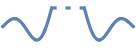
By default, the real and imaginary parts are solid and dashed, respectively:
ReImPlot[{ArcSin[x], ArcCos[x]}, {x, -3, 3}]Modify the real and imaginary styles:
ReImPlot[{ArcSin[x], ArcCos[x]}, {x, -3, 3}, ReImStyle -> {Thickness[.02], Dashing[{0.03, 0.01}]}]Applications (7)
ft = FourierTransform[Exp[-x]UnitStep[x], x, k];ReImPlot[ft, {k, -5, 5}]Plot the solution of a complex differential equation with initial conditions:
sol = NDSolveValue[{y''[x] - I Sin[y[x]] == 0, y[0] == 1, y'[0] == 2}, y[x], {x, 0, 10}];ReImPlot[sol, {x, 0, 10}, PlotRange -> All]Plot the eigenvalues of a matrix as a function of a parameter:
ReImPlot[Eigenvalues[{{b - 1, 1}, {-b, -1}}], {b, -2, 6}]Plot solutions of an equation as a function of a parameter:
ReImPlot[Evaluate[x /. Solve[a + 2x^2 - x^3 == 0, x]], {a, -3, 3}, PlotLegends -> {"Expressions", "ReIm"}]ReImPlot[JacobiZeta[x, 10], {x, -2Pi, 2Pi}, Ticks -> {Range[-2Pi, 2Pi, Pi / 2], Automatic}, PlotLegends -> "AllExpressions"]Plot fractional derivatives of ![]() :
:
Grid[Partition[Table[ReImPlot[{x^2, (Gamma[2 + 1]/Gamma[2 - b + 1])x^2 - b}, {x, -5, 5}, PlotRange -> {-10, 10}, PlotLabel -> Derivative[b][y][x]], {b, 1 / 3, 3, 1 / 3}], 3], Dividers -> All]Plot the complex solution of the Schrödinger equation for a particle in a box:
Manipulate[
	ReImPlot[Sqrt[2] E^-(1/2) I n^2 π^2 t Sin[n π x], {x, 0, 1}, PlotRange -> {-2, 2}, AxesLabel -> {(x/L), Sqrt[L]ψ}],
	{{t, 0, (ℏ π^2/2m L^2)t}, 0, (4/n^2π)}, {{n, 3}, 1, 10, 1}]
Properties & Relations (8)
ReImPlot is a special case of Plot:
{Plot[ReIm[ArcSin[x]], {x, -3, 3}],
	ReImPlot[ArcSin[x], {x, -3, 3}]}
Use AbsArgPlot to plot the magnitude and argument over the real numbers:
AbsArgPlot[Log[x], {x, -3, 3}]ComplexPlot shows the argument and magnitude of a function using color:
ComplexPlot[Log[z], {z, 3}]Use ComplexPlot3D to use the z axis for the magnitude:
ComplexPlot3D[Log[z], {z, 3}]Use ComplexListPlot to show the location of complex numbers in the plane:
ComplexListPlot[RandomComplex[{-3 - 3I, 3 + 3I}, 100]]ComplexContourPlot plots curves over the complexes:
ComplexContourPlot[Abs[Log[z]] == 1, {z, 3}]ComplexRegionPlot plots regions over the complexes:
ComplexRegionPlot[Abs[Log[z]] < 1, {z, 3}]ComplexStreamPlot and ComplexVectorPlot treat complex numbers as directions:
ComplexStreamPlot[Log[z], {z, 3}]ComplexVectorPlot[Log[z], {z, 3}]Possible Issues (1)
ScalingFunctions applies to the real and imaginary parts:
ReImPlot[Exp[t] + I t, {t, -3π, 3π}, ScalingFunctions -> "Log"]Text
Wolfram Research (2019), ReImPlot, Wolfram Language function, https://reference.wolfram.com/language/ref/ReImPlot.html (updated 2023).
CMS
Wolfram Language. 2019. "ReImPlot." Wolfram Language & System Documentation Center. Wolfram Research. Last Modified 2023. https://reference.wolfram.com/language/ref/ReImPlot.html.
APA
Wolfram Language. (2019). ReImPlot. Wolfram Language & System Documentation Center. Retrieved from https://reference.wolfram.com/language/ref/ReImPlot.html