DiscretePlot3D[f,{i,imin,imax},{j,jmin,jmax}]
i の範囲が iminから imaxまで,j の範囲が jminから jmaxまでの,f の値のプロットを生成する.
DiscretePlot3D[f,{i,imin,imax,di},{j,jmin,jmax,dj}]
ステップ di と dj を使う.
DiscretePlot3D[f,{i,{i1,…,im}},{j,{j1,…,jn}}]
連続する i の値 i1, …, jmと j の値 j1, …, jnを使う.
DiscretePlot3D[{f1,f2,…},…,…]
fkのすべての値をプロットする.
DiscretePlot3D
DiscretePlot3D[f,{i,imin,imax},{j,jmin,jmax}]
i の範囲が iminから imaxまで,j の範囲が jminから jmaxまでの,f の値のプロットを生成する.
DiscretePlot3D[f,{i,imin,imax,di},{j,jmin,jmax,dj}]
ステップ di と dj を使う.
DiscretePlot3D[f,{i,{i1,…,im}},{j,{j1,…,jn}}]
連続する i の値 i1, …, jmと j の値 j1, …, jnを使う.
DiscretePlot3D[{f1,f2,…},…,…]
fkのすべての値をプロットする.
詳細とオプション
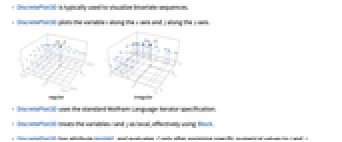
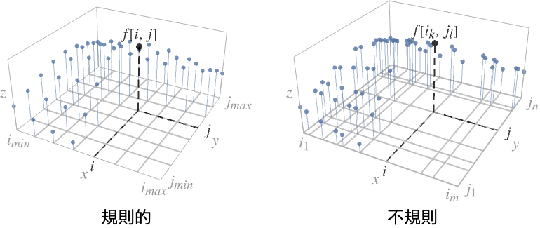
- DiscretePlot3Dは,通常,二変量の数列を可視化するために使われる.
- DiscretePlot3Dは,変数 i を
軸に沿って,変数 j を
軸に沿ってプロットする. - DiscretePlot3Dは標準的なWolfram言語の反復子指定を使う.
- DiscretePlot3Dは事実上Blockを使って変数 i,j を局所的なものとして扱う.
- DiscretePlot3Dは属性HoldAllを有し,i と j に特定の数値を割り当てた後ではじめて f を評価する.
- 場合によっては,i と j に特定の数値を割り当てる前にEvaluateを使って f を記号的に評価する方が効率がよい場合もある.
- f の評価に使われる精度は反復子が使う最低精度である.
- 結果のグラフィックスプリミティブに適用されるラッパー w は w[f]の形で与えられる.
- 使用可能なラッパー
-
Annotation[f,label] 注釈を与える Button[f,action] 要素がクリックされたときのアクションを定義する Callout[f,label] コールアウトで要素にラベルを付ける Callout[f,label,pos] コールアウトを相対的な位置 pos に置く EventHandler[f,…] 要素の一般的なイベントハンドラを定義する Hyperlink[f,uri] 要素をハイパーリンクにする Labeled[f,label] データをハイパーリンクにする Labeled[f,label,pos] ラベルを相対的な位置 pos に置く Legended[f,label] 凡例中の要素を識別する PopupWindow[f,cont] 要素にポップアップウィンドウを付加する StatusArea[f,label] 要素上にマウスが置かれたときにステータスエリアに表示っする Style[f,opts] 指定のスタイルで要素を表示する Tooltip[f,label] 要素に任意のツールチップを付加する - CalloutおよびLabeledは次の位置 pos を使うことができる.
-
Automatic ラベルを自動的に置く Above, Below, Before, After データの周りの位置 x 位置 x におけるデータの近く {s,Above},{s,Below},… データに沿った位置 s と相対的な位置 {pos,epos} データの相対的な位置 pos に置かれたラベル内の epos - {i,j}に依存するラベルは各プロット要素に適用されるのに対し,{i,j}に依存しないラベルは1回だけ出現する.
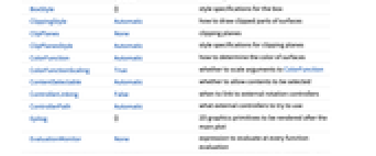
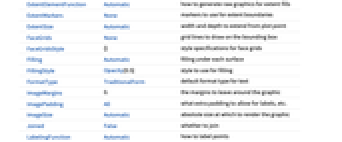
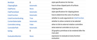
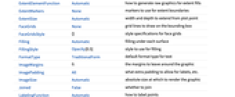
- DiscretePlot3DにはGraphics3Dと同じオプションに次の追加・変更を加えたものが使える. [全オプションのリスト]
-
Axes True 座標軸を描くかどうか BoxRatios {1,1,0.4} 境界3Dボックス比 ClippingStyle Automatic 曲面の切り取られた部分をどのように描くか ColorFunction Automatic 曲面の色の決め方 ColorFunctionScaling True ColorFunctionの引数をスケールするかどうか EvaluationMonitor None すべての関数評価で評価する式 ExtentElementFunction Automatic 範囲を埋めるための生の画像の生成方法 ExtentMarkers None 境界範囲を示すマーカー ExtentSize Automatic プロットポイントから延長する幅と深さ Filling Automatic 各曲面の下の充填 FillingStyle Opacity[0.5] 充填に使うスタイル Joined False 繋ぐかどうか LabelingFunction Automatic 点にどのようにラベルを付けるか LabelingSize Automatic コールアウトとラベルの最大サイズ Method Automatic 使用するメソッド PerformanceGoal $PerformanceGoal パフォーマンスのどの面について最適化するか PlotLegends None 数列のための凡例 PlotMarkers None プロットの点に使うマーカー PlotRange {Full,Full,Automatic} 含める
やその他の値の範囲PlotStyle Automatic 各曲面のスタイルのためのグラフィックス指示子 PlotTheme $PlotTheme プロットの全体的なテーマ RegionFunction (True&) 点を含めるかどうかの決め方 ScalingFunctions None 個々の座標をどのようにスケールするか WorkingPrecision MachinePrecision 内部計算に使う精度 - ColorFunctionに渡される引数は,
,
,
である. - ExtentSize->{{sxl,sxr},{syl,syr}}と設定すると,
軸に沿って sxlを左に sxrを右に,
軸に沿って sylを左に syrを右に延長して各プロット点の周りに水平面が描かれる.ExtentMarkers->{{mxl,mxr},{myl,myr}}とすると,
軸に沿った左右のマーカーとして mxlと mxrが,
軸に沿った左右のマーカーとして mylと myrが使われる. - ExtentElementFunctionに渡される引数は要素範囲{{xmin,xmax},{ymin,ymax},{zmin,zmax}}とサンプル点{xi,yi,zi}である.
- ExtentSize->Noneと設定すると,xminと xmaxは等しくなり,yminと ymaxも等しくなる.Filling->Noneとすると,zminは zmaxと等しくなる.
- 次は,PlotMarkersの可能な設定である.
-
None 曲面を描画する際にはマーカーを省略する "Point" 2Dの点をマーカーとして使う "Sphere" 3Dの曲面をマーカーとして使う {"Point",s},{"Sphere",s} マーカーサイズ s を指定する {spec1,spec2,…} 式 expriに指定 speciを使う - マーカーのサイズ s は,Tiny,Small,Medium,Large等の記号による値,あるいはグラフィックスの幅とのスケールされた割合でよい.
- 次は,ScalingFunctionsの可能な設定である.
-
sz z 軸をスケールする {sx,sy} x 軸と y 軸をスケールする {sx,sy,sz} x, y, z 軸をスケールする - 各スケーリング関数 siは文字列"scale"または{g,g-1}である.ここで,g-1は g の逆関数である.
全オプションのリスト
例題
すべて開く すべて閉じる例 (3)
DiscretePlot3D[PDF[MultivariatePoissonDistribution[3, {1, 1}], {t, u}], {t, 0, 10}, {u, 0, 10}]DiscretePlot3D[PDF[MultivariatePoissonDistribution[3, {1, 1}], {t, u}], {t, 0, 10}, {u, 0, 10}, ExtentSize -> Full]DiscretePlot3D[{PDF[MultivariatePoissonDistribution[3, {1, 1}], {t, u}], PDF[MultivariatePoissonDistribution[5, {2, 2}], {t, u}]}, {t, 0, 10}, {u, 0, 10}, ExtentSize -> Full]スコープ (12)
データとレイアウト (4)
DiscretePlot3D[{Sin[t + u], Cos[t + u]}, {t, 0, 2Pi, Pi / 12}, {u, 0, 2Pi, Pi / 12}, ExtentSize -> Full]個々のデータ,データ集合,あるいはデータ集合の集合にラッパーを使う:
{DiscretePlot3D[{Sin[t + u], Cos[t + u]}, {t, 0, 2 * Pi, Pi / 6}, {u, 0, 2 * Pi, Pi / 6}, ExtentSize -> Full], DiscretePlot3D[{Sin[t + u], Style[Cos[t + u], Green]}, {t, 0, 2 * Pi, Pi / 6}, {u, 0, 2 * Pi, Pi / 6}, ExtentSize -> Full], DiscretePlot3D[Style[{Sin[t + u], Cos[t + u]}, Green], {t, 0, 2 * Pi, Pi / 6}, {u, 0, 2 * Pi, Pi / 6}, ExtentSize -> Full]}DiscretePlot3D[Style[{Sin[t + u], Style[Cos[t + u], Green]}, Red], {t, 0, 2 * Pi, Pi / 12}, {u, 0, 2 * Pi, Pi / 12}, ExtentSize -> Full]DiscretePlot3D[{Sin[t + u], Tooltip[Cos[t + u], "my data"]}, {t, 0, 2 * Pi, Pi / 12}, {u, 0, 2 * Pi, Pi / 12}, ExtentSize -> Full]PopupWindowを使って追加的なドリルダウンの情報を加える:
DiscretePlot3D[PopupWindow[PDF[MultivariatePoissonDistribution[3, {1, 1}], {t, u}], TraditionalForm[PDF[MultivariatePoissonDistribution[3, {1, 1}], {t, u}]]], {t, 0, 10}, {u, 0, 10}, ExtentSize -> Full]Buttonを使ってアクションを起すことができる:
DiscretePlot3D[Evaluate@Table[With[{lambda = λ}, Button[PDF[
MultivariatePoissonDistribution[lambda, {1, 1}], {t, u}],
Speak[MultivariatePoissonDistribution[lambda, {1, 1}]]]], {λ, {1, 2, 3}}],
{t, 0, 10}, {u, 0, 10}, PlotRange -> All, ExtentSize -> Full]ScalingFunctionsを使って軸をスケールする:
DiscretePlot3D[LCM[x, y], {x, 20}, {y, 20}, ExtentSize -> Full, ScalingFunctions -> "Log"]ラベル付けと凡例 (3)
DiscretePlot3D[Callout[GCD[x, y], If[x == y, x, None], Above], {x, Prime[Range[10]]}, {y, Prime[Range[10]]}]DiscretePlot3D[Tooltip[GCD[x, y], GCD[x, y]], {x, Prime[Range[10]]}, {y, Prime[Range[10]]}]LabelingFunctionでラベル名を指定する:
DiscretePlot3D[GCD[x, y], {x, 1, 5}, {y, 1, 5}, LabelingFunction -> (#1[[1]] &)]DiscretePlot3D[Callout[GCD[x, y], IntegerName@GCD[x, y]], {x, 1, 5}, {y, 1, 5}]スタイルと外観 (5)
ExtentSizeを使って範囲と点を関連付ける:
Table[DiscretePlot3D[PDF[MultivariatePoissonDistribution[3, {1, 1}], {t, u}], {t, 0, 10}, {u, 0, 10}, ExtentSize -> s, PlotLabel -> s], {s, {None, Full, Right, Scaled[0.5]}}]DiscretePlot3D[{Sin[t + u], Cos[t + u]}, {t, 0, 2 * Pi}, {u, 0, 2 * Pi}, PlotStyle -> {Red, Blue}, ExtentSize -> Full]ColorDataから任意の階調度カラースキームを使う:
{DiscretePlot3D[{Sin[t + u], Cos[t + u]}, {t, 0, 2 * Pi}, {u, 0, 2 * Pi}, ColorFunction -> "Pastel", ExtentSize -> Full], DiscretePlot3D[{Sin[t + u], Cos[t + u]}, {t, 0, 2 * Pi}, {u, 0, 2 * Pi}, ColorFunction -> Function[{x, y}, ColorData["NeonColors"][y]], ExtentSize -> Full]}Styleを使ってスタイルを無効にすることができる:
DiscretePlot3D[{Sin[t + u], Style[Cos[t + u], Red]}, {t, 0, 2 * Pi}, {u, 0, 2 * Pi}, PlotStyle -> Gray, ExtentSize -> Full]DiscretePlot3D[Exp[-x ^ 2 - y ^ 2], {x, -3, 3, 0.25}, {y, -3, 3, 0.25}, PlotMarkers -> "Sphere"]DiscretePlot3D[PDF[MultivariatePoissonDistribution[3, {1, 1}], {t, u}], {t, 10}, {u, 10}, ColorFunction -> "Rainbow", ExtentSize -> Full, ExtentMarkers -> "Tube"]DiscretePlot3D[PDF[MultivariatePoissonDistribution[3, {1, 1}], {t, u}], {t, 10}, {u, 10}, ExtentSize -> Full, ColorFunction -> "DarkRainbow", ExtentMarkers -> {{"Tube", None}, {"Tube", None}}]暗い背景でコントラストがはっきりしたカラースキームのテーマを使う:
DiscretePlot3D[Mod[x, y], {x, 10}, {y, 10}, PlotTheme -> "Marketing"]オプション (90)
Axes (3)
デフォルトで,DiscretePlot3DにはAxesが描かれる:
DiscretePlot3D[Mod[x, y], {x, 10}, {y, 10}, ExtentSize -> Full]DiscretePlot3D[Mod[x, y], {x, 10}, {y, 10}, ExtentSize -> Full, Axes -> False]{DiscretePlot3D[Mod[x, y], {x, 10}, {y, 10}, ExtentSize -> Full, Axes -> {True, False, False}], DiscretePlot3D[Mod[x, y], {x, 10}, {y, 10}, ExtentSize -> Full, Axes -> {False, True, False}], DiscretePlot3D[Mod[x, y], {x, 10}, {y, 10}, ExtentSize -> Full, Axes -> {False, False, True}]}AxesLabel (4)
DiscretePlot3D[Mod[x, y], {x, 10}, {y, 10}, ExtentSize -> Full]DiscretePlot3D[Mod[x, y], {x, 10}, {y, 10}, ExtentSize -> Full, AxesLabel -> "Mod[x,y]"]DiscretePlot3D[Mod[x, y], {x, 10}, {y, 10}, ExtentSize -> Full, AxesLabel -> {"x", "y", "Mod[x,y]"}]DiscretePlot3Dで指定された変数に基づくラベルを使う:
DiscretePlot3D[Mod[x, y], {x, 10}, {y, 10}, ExtentSize -> Full, AxesLabel -> Automatic]AxesOrigin (2)
AxesStyle (4)
DiscretePlot3D[Mod[x, y], {x, 10}, {y, 10}, ExtentSize -> Full, AxesStyle -> Red]DiscretePlot3D[Mod[x, y], {x, 10}, {y, 10}, ExtentSize -> Full, AxesStyle -> {{Thick, Brown}, {Thick, Blue}, {Thick, Green}}]DiscretePlot3D[Mod[x, y], {x, 10}, {y, 10}, ExtentSize -> Full, AxesStyle -> Green, TicksStyle -> StandardBlue]DiscretePlot3D[Mod[x, y], {x, 10}, {y, 10}, ExtentSize -> Full, AxesStyle -> Green, LabelStyle -> Red]ColorFunction (6)
Map[DiscretePlot3D[PDF[MultivariatePoissonDistribution[5, {2, 3}], {x, y}], {x, 0, 15}, {y, 0, 15}, ColorFunction -> Function[{x, y, z}, #], PlotLabel -> #]&, {Hue[x], Hue[y], Hue[z]}]Map[DiscretePlot3D[PDF[MultivariatePoissonDistribution[5, {2, 3}], {x, y}], {x, 0, 15}, {y, 0, 15}, Joined -> True, PlotRange -> All, ColorFunction -> Function[{x, y, z}, #], PlotLabel -> #]&, {Hue[x], Hue[y], Hue[z]}]Map[DiscretePlot3D[PDF[MultivariatePoissonDistribution[5, {2, 3}], {x, y}], {x, 0, 15}, {y, 0, 15}, ExtentSize -> Full, ColorFunction -> Function[{x, y, z}, #], PlotLabel -> #]&, {Hue[x], Hue[y], Hue[z]}]DiscretePlot3D[PDF[MultivariatePoissonDistribution[1, {1, 1}], {x, y}], {x, 0, 15}, {y, 0, 15}, ExtentSize -> Full, ColorFunction -> "Rainbow"]ColorFunctionはPlotStyleより優先順位が高い:
DiscretePlot3D[PDF[MultivariatePoissonDistribution[5, {2, 3}], {x, y}], {x, 0, 15}, {y, 0, 15}, ColorFunction -> "Rainbow", PlotStyle -> Directive[Red, PointSize[Large]]]DiscretePlot3D[GCD[m, n], {m, 1, 20}, {n, 1, 20}, ExtentSize -> Full, ColorFunction -> Function[{x, y, z}, If[z == 1, Black, Hue[z / 20]]], ColorFunctionScaling -> False]ColorFunctionScaling (1)
EvaluationMonitor (1)
ExtentElementFunction (5)
ExtentElementFunctionの組込み設定のリストを得る:
ChartElementData["DiscretePlot3D"]詳細設定には「パレット」▶「チャートエレメントスキーム」を使う:
Table[DiscretePlot3D[PDF[MultivariatePoissonDistribution[1, {1, 1}], {x, y}], {x, 0, 8}, {y, 0, 8}, ExtentSize -> Full, ExtentElementFunction -> f], {f, {"Cone", "Cube", "Cylinder", "PlaneFadingCube"}}]Table[DiscretePlot3D[PDF[MultivariatePoissonDistribution[1, {1, 1}], {x, y}], {x, 0, 8}, {y, 0, 8}, ExtentSize -> Full, ExtentElementFunction -> f], {f, {"ProfileCube", "DoubleProfileCube", "SquareWaveCube", "TriangleWaveCube"}}]ChartElementFunctionは大域スケールを示すのに相応しい:
Table[DiscretePlot3D[PDF[MultivariatePoissonDistribution[1, {1, 1}], {x, y}], {x, 0, 8}, {y, 0, 8}, ExtentSize -> Full, ExtentElementFunction -> f], {f, {"GradientScaleCube", "SegmentScaleCube"}}]カスタムExtentElementFunctionを書く:
vase[{{xmin_, xmax_}, {ymin_, ymax_}, {zmin_, zmax_}}, ___] := {CapForm[None], Tube[
Table[{(xmin + xmax) / 2, (ymin + ymax) / 2, z}, {z, zmin, zmax, (zmax - zmin) / 15}],
Join[Sort[RandomReal[(xmax - xmin){0.1, 0.5}, 8], Less], Sort[RandomReal[(xmax - xmin){0.1, 0.5}, 8], Greater]]]}DiscretePlot3D[PDF[MultivariatePoissonDistribution[1, {1, 1}], {x, y}], {x, 0, 5}, {y, 0, 5}, ExtentSize -> Full, ExtentElementFunction -> vase, PlotRange -> {0, 0.1}]組込み要素にはオプションがあることがある.「パレット」▶「チャートエレメントスキーム」を使ってオプションを設定する:
ChartElementData["ProfileCube", "Options"]Table[DiscretePlot3D[PDF[MultivariatePoissonDistribution[1, {1, 1}], {x, y}], {x, 0, 5}, {y, 0, 5}, ExtentSize -> Full, ExtentElementFunction -> ChartElementData["ProfileCube", "Profile" -> p, "TaperRatio" -> r]], {p, {0.1, 1, 5}}, {r, {0, 0.5, 1}}]ExtentMarkers (4)
DiscretePlot3D[LCM[m, n], {m, 6}, {n, 6}, ExtentSize -> Full, ExtentMarkers -> None, PlotStyle -> EdgeForm[]]DiscretePlot3D[LCM[m, n], {m, 6}, {n, 6}, ExtentSize -> Full, ExtentMarkers -> {"Line", 5}, PlotStyle -> EdgeForm[]]Table[DiscretePlot3D[LCM[m, n], {m, 5}, {n, 5}, ExtentSize -> Full, ExtentMarkers -> {"Tube", size}], {size, {Tiny, Small, Medium, Large}}]DiscretePlot3D[LCM[m, n], {m, 5}, {n, 5}, ExtentSize -> Full, ExtentMarkers -> {{"Tube", None}, {"Tube", None}}]ExtentSize (6)
DiscretePlot3D[LCM[m, n], {m, 5}, {n, 5}, ExtentSize -> None]DiscretePlot3D[LCM[m, n], {m, 5}, {n, 5}, ExtentSize -> Full]DiscretePlot3D[LCM[m, n], {m, {1, 2, 3, 5, 8, 13}}, {n, {1, 2, 3, 5, 8, 13}}, ExtentSize -> Full]DiscretePlot3D[LCM[m, n], {m, 5}, {n, 5}, ExtentSize -> 0.5]DiscretePlot3D[LCM[m, n], {m, {1, 2, 3, 5, 8, 13}}, {n, {1, 2, 3, 5, 8, 13}}, ExtentSize -> 0.5]DiscretePlot3D[LCM[m, n], {m, 5}, {n, 5}, ExtentSize -> Scaled[0.75]]DiscretePlot3D[LCM[m, n], {m, {1, 2, 3, 5, 8, 13}}, {n, {1, 2, 3, 5, 8, 13}}, ExtentSize -> Scaled[0.75]]DiscretePlot3D[LCM[m, n], {m, 5}, {n, 5}, ExtentSize -> All]DiscretePlot3D[LCM[m, n], {m, {1, 2, 3, 5, 8, 13}}, {n, {1, 2, 3, 5, 8, 13}}, ExtentSize -> All]Table[DiscretePlot3D[LCM[m, n], {m, 5}, {n, 5}, ExtentSize -> es, PlotLabel -> es, PlotMarkers -> {"Sphere", Large}], {es, {{{None, Full}, {None, Full}}, {{Full, None}, {Full, None}}}}]Filling (3)
DiscretePlot3Dは
まで埋める:
Table[DiscretePlot3D[Mod[m, n], {m, 15}, {n, 15}, Evaluate[opt]], {opt, {Joined -> False, Joined -> True, ExtentSize -> Full}}]Table[DiscretePlot3D[Mod[m, n], {m, 15}, {n, 15}, Filling -> None, Evaluate[opt]], {opt, {Joined -> False, Joined -> True, ExtentSize -> Full}}]Table[DiscretePlot3D[Mod[m, n] - Mod[n, m], {m, 15}, {n, 15}, Filling -> fill, PlotLabel -> fill], {fill, {Bottom, Top, Axis, -20}}]FillingStyle (3)
Table[DiscretePlot3D[Mod[m, n] - Mod[n, m], {m, 15}, {n, 15}, Filling -> Bottom, FillingStyle -> fs], {fs, {Opacity[1], Red, Dashed, Thick}}]Table[DiscretePlot3D[Mod[m, n] - Mod[n, m], {m, 15}, {n, 15}, ExtentSize -> Full, Filling -> Bottom, FillingStyle -> fs], {fs, {Opacity[1], Red}}]Table[DiscretePlot3D[Mod[m, n] - Mod[n, m], {m, 15}, {n, 15}, ExtentSize -> es, Filling -> Axis, FillingStyle -> {Red, Blue}], {es, {None, Full}}]Table[DiscretePlot3D[Mod[m, n] - Mod[n, m], {m, 15}, {n, 15}, ExtentSize -> es, Filling -> Axis, FillingStyle -> {Red, None}], {es, {None, Full}}]ImageSize (7)
Tiny,Small,Medium,Largeのような名前付きのサイズを使う:
{DiscretePlot3D[Mod[x, y], {x, 10}, {y, 10}, ExtentSize -> Full, ImageSize -> Tiny], DiscretePlot3D[Mod[x, y], {x, 10}, {y, 10}, ExtentSize -> Full, ImageSize -> Small]}{DiscretePlot3D[Mod[x, y], {x, 10}, {y, 10}, ExtentSize -> Full, ImageSize -> 150], DiscretePlot3D[Mod[x, y], {x, 10}, {y, 10}, ExtentSize -> Full, AspectRatio -> 1.5, ImageSize -> 150]}{DiscretePlot3D[Mod[x, y], {x, 10}, {y, 10}, ExtentSize -> Full, ImageSize -> {Automatic, 150}], DiscretePlot3D[Mod[x, y], {x, 10}, {y, 10}, ExtentSize -> Full, AspectRatio -> 2, ImageSize -> {Automatic, 150}]}{DiscretePlot3D[Mod[x, y], {x, 10}, {y, 10}, ExtentSize -> Full, ImageSize -> UpTo[200]], DiscretePlot3D[Mod[x, y], {x, 10}, {y, 10}, ExtentSize -> Full, AspectRatio -> 2, ImageSize -> UpTo[200]]}グラフィックスの幅と高さを指定し,必要な場合はスペースで充填する:
DiscretePlot3D[Mod[x, y], {x, 10}, {y, 10}, ExtentSize -> Full, ImageSize -> {200, 250}, Background -> StandardGray]AspectRatioFullと設定すると使用可能なスペースが塗り潰される:
DiscretePlot3D[Mod[x, y], {x, 10}, {y, 10}, ExtentSize -> Full, AspectRatio -> Full, ImageSize -> {200, 250}, Background -> StandardGray]{DiscretePlot3D[Mod[x, y], {x, 10}, {y, 10}, ExtentSize -> Full, ImageSize -> {UpTo[150], UpTo[100]}], DiscretePlot3D[Mod[x, y], {x, 10}, {y, 10}, ExtentSize -> Full, AspectRatio -> 2, ImageSize -> {UpTo[150], UpTo[100]}]}ImageSizeFullを使ってオブジェクト内の使用可能なスペースを塗り潰す:
Framed[Pane[DiscretePlot3D[Mod[x, y], {x, 10}, {y, 10}, ExtentSize -> Full, ImageSize -> Full, Background -> StandardGray], {200, 100}]]Framed[Pane[DiscretePlot3D[Mod[x, y], {x, 10}, {y, 10}, ExtentSize -> Full, AspectRatio -> Full, ImageSize -> {Scaled[0.5], Scaled[0.5]}, Background -> StandardGray], {250, 250}]]Joined (2)
DiscretePlot3D[PDF[MultivariatePoissonDistribution[5, {2, 3}], {x, y}], {x, 0, 15}, {y, 0, 15}, Joined -> True]DiscretePlot3D[PDF[MultivariatePoissonDistribution[5, {2, 3}], {x, y}], {x, 0, 15}, {y, 0, 15}, Joined -> True, ExtentSize -> Full]LabelingFunction (4)
DiscretePlot3D[GCD[x, y], {x, 1, 5}, {y, 1, 5}, LabelingFunction -> Above]DiscretePlot3D[GCD[x, y], {x, 1, 5}, {y, 1, 5}, LabelingFunction -> Tooltip]DiscretePlot3D[GCD[x, y], {x, 1, 5}, {y, 1, 5}, LabelingFunction -> Callout[Automatic, Automatic]]DiscretePlot3D[GCD[x, y], {x, 1, 5}, {y, 1, 5}, LabelingFunction -> (#1&)]DiscretePlot3D[GCD[x, y], {x, 1, 5}, {y, 1, 5}, LabelingFunction -> (#2&)]LabelingSize (1)
DiscretePlot3D[Callout[GCD[x, y], IntegerName[x]], {x, 500, 505}, {y, 500, 505}, ImageSize -> Medium, LabelingSize -> 30]DiscretePlot3D[Callout[x + y, IntegerName[x + y]], {x, 0, 10}, {y, 0, 10}, ImageSize -> Medium, LabelingSize -> Full]PlotLegends (6)
DiscretePlot3D[{Sin[x + y], Cos[x + y]}, {x, 20}, {y, 20}, ExtentSize -> Full, PlotLegends -> Automatic]DiscretePlot3D[{x, y}, {x, 20}, {y, 20}, ExtentSize -> Full, PlotLegends -> {"label1", "label2"}]DiscretePlot3D[{Sin[x + y], Sin[x - y]}, {x, 20}, {y, 20}, ExtentSize -> Full, PlotLegends -> "Expressions"]PlotLegendsは自動的にPlotStyleの値を取る:
DiscretePlot3D[{Sin[(x + y) ^ 2], Sin[(x - y) ^ 2]}, {x, 0, 2, 0.2}, {y, 0, 2, 0.2}, ExtentSize -> Full, PlotStyle -> {Red, Blue}, PlotLegends -> "Expressions"]Placedを使って凡例の置き方を制御する:
Table[DiscretePlot3D[{Sin[(x + y)], Sin[(x - y)]}, {x, 0, 2, 0.2}, {y, 0, 2, 0.2}, ExtentSize -> Full, PlotStyle -> {Orange, Blue}, PlotLegends -> Placed["Expressions", pos]], {pos, {Above, Below}}]SwatchLegendを使って凡例の外観を変える:
DiscretePlot3D[{Sin[(x + y) ^ 2], Sin[(x - y) ^ 2]}, {x, 0, 2, 0.2}, {y, 0, 2, 0.2}, ExtentSize -> Full, PlotStyle -> {Red, Blue}, PlotLegends -> SwatchLegend["Expressions", LegendLabel -> "label", LegendFunction -> (Framed[#, RoundingRadius -> 5]&)]]PlotMarkers (4)
Table[DiscretePlot3D[PDF[MultivariatePoissonDistribution[5, {2, 3}], {x, y}], {x, 0, 15}, {y, 0, 15}, PlotMarkers -> {Automatic, s}], {s, {Tiny, Small, Medium, Large}}]{DiscretePlot3D[PDF[MultivariatePoissonDistribution[5, {2, 3}], {x, y}], {x, 0, 15}, {y, 0, 15}, Joined -> True], DiscretePlot3D[PDF[MultivariatePoissonDistribution[5, {2, 3}], {x, y}], {x, 0, 15}, {y, 0, 15}, ExtentSize -> Full]}{DiscretePlot3D[PDF[MultivariatePoissonDistribution[5, {2, 3}], {x, y}], {x, 0, 15}, {y, 0, 15}, Joined -> True, PlotMarkers -> "Point", PlotStyle -> FaceForm[Lighter[Blue, 0.5]]], DiscretePlot3D[PDF[MultivariatePoissonDistribution[5, {2, 3}], {x, y}], {x, 0, 15}, {y, 0, 15}, ExtentSize -> Full, PlotMarkers -> "Point"]}{DiscretePlot3D[PDF[MultivariatePoissonDistribution[5, {2, 3}], {x, y}], {x, 0, 15}, {y, 0, 15}, PlotMarkers -> "Sphere"], DiscretePlot3D[PDF[MultivariatePoissonDistribution[5, {2, 3}], {x, y}], {x, 0, 15}, {y, 0, 15}, ExtentSize -> Full, PlotMarkers -> "Sphere"]}Table[DiscretePlot3D[PDF[MultivariatePoissonDistribution[5, {2, 3}], {x, y}], {x, 0, 15}, {y, 0, 15}, PlotMarkers -> {"Sphere", s}], {s, {Tiny, Small, Medium, Large}}]PlotStyle (7)
Table[DiscretePlot3D[PDF[MultivariatePoissonDistribution[5, {2, 3}], {x, y}], {x, 0, 15}, {y, 0, 15}, PlotStyle -> ps], {ps, {Red, PointSize[0.025], Darker[Green], Directive[Red, PointSize[Small]]}}]DiscretePlot3D[Evaluate[Table[PDF[MultivariatePoissonDistribution[2k, {k, 3k}], {x, y}], {k, 3}]], {x, 20}, {y, 20}, ExtentSize -> Full]DiscretePlot3D[Evaluate[Table[PDF[MultivariatePoissonDistribution[2k, {k, 3k}], {x, y}], {k, 3}]], {x, 20}, {y, 20}, ExtentSize -> Full, PlotStyle -> {Red, Orange, Blue}]PlotStyleは点,線,曲面に適用される:
DiscretePlot3D[PDF[MultivariatePoissonDistribution[5, {2, 3}], {x, y}], {x, 0, 15}, {y, 0, 15}, PlotStyle -> Red]DiscretePlot3D[PDF[MultivariatePoissonDistribution[5, {2, 3}], {x, y}], {x, 0, 15}, {y, 0, 15}, ExtentSize -> Full, PlotStyle -> Directive[Orange, EdgeForm[Blue]]]PlotStyleはColorFunctionと組み合せることができる:
DiscretePlot3D[PDF[MultivariatePoissonDistribution[5, {2, 3}], {x, y}], {x, 0, 15}, {y, 0, 15}, PlotStyle -> PointSize[Medium], ColorFunction -> Function[{x, y, z}, Hue[z]]]PlotStyleはFillingStyleと組み合せることができる:
DiscretePlot3D[PDF[MultivariatePoissonDistribution[5, {2, 3}], {x, y}], {x, 0, 15}, {y, 0, 15}, PlotStyle -> Red, FillingStyle -> Opacity[1]]FillingStyleはデフォルトでPlotStyleと同じスタイルを透明度を持たせて使う:
DiscretePlot3D[PDF[MultivariatePoissonDistribution[5, {2, 3}], {x, y}], {x, 0, 15}, {y, 0, 15}, PlotStyle -> Red]PlotTheme (4)
DiscretePlot3D[{CDF[MultivariatePoissonDistribution[3, {1, 1}], {t, u}], SurvivalFunction[MultivariatePoissonDistribution[3, {1, 1}], {t, u}]}, {t, 10}, {u, 10}, PlotTheme -> "Business"]DiscretePlot3D[{CDF[MultivariatePoissonDistribution[3, {1, 1}], {t, u}], SurvivalFunction[MultivariatePoissonDistribution[3, {1, 1}], {t, u}]}, {t, 10}, {u, 10}, PlotTheme -> "Business", PlotStyle -> {Red, Blue}]暗い背景でコントラストのはっきりしたカラースキームのテーマを使う:
DiscretePlot3D[GCD[m, n], {m, 15}, {n, 15}, PlotTheme -> "Marketing"]DiscretePlot3D[GCD[m, n], {m, 15}, {n, 15}, PlotTheme -> "Marketing", Ticks -> None]RegionFunction (4)
DiscretePlot3D[GCD[m, n], {m, 25}, {n, 25}, RegionFunction -> Function[{m, n, z}, m ≤ n]]拡大された領域は追加的な切取りなしで基になっている点として扱われる:
DiscretePlot3D[GCD[m, n], {m, 5}, {n, 5}, ExtentSize -> Full, RegionFunction -> Function[{m, n, z}, m <= n], PlotMarkers -> "Sphere"]DiscretePlot3D[GCD[m, n], {m, 25}, {n, 25}, RegionFunction -> Function[{m, n, z}, Mod[m + n, 10] ≤ 7]]DiscretePlot3D[GCD[m, n], {m, 25}, {n, 25}, RegionFunction -> Function[{m, n, z}, m ^ 2 + n ^ 2 ≤ 625 && m + n ≥ 25]]ScalingFunctions (9)
DiscretePlot3D[Max[x, y], {x, 0, 10, .5}, {y, 0, 10, .5}, ExtentSize -> Full]DiscretePlot3D[Max[x, y], {x, 1, 10, .5}, {y, 1, 10, .5}, ExtentSize -> Full, ScalingFunctions -> "Log"]DiscretePlot3D[Max[x, y], {x, 0, 10, .5}, {y, 0, 10, .5}, ExtentSize -> Full, ScalingFunctions -> {None, "Reverse"}]DiscretePlot3D[Max[x, y], {x, 1, 10, .5}, {y, 1, 10, .5}, ExtentSize -> Full, ScalingFunctions -> {None, "Reciprocal"}]DiscretePlot3D[Max[x, y], {x, 0, 10, .5}, {y, 0, 10, .5}, ExtentSize -> Full, ScalingFunctions -> {"Reverse", "Log"}]DiscretePlot3D[Max[x, y], {x, 0, 10, .5}, {y, 0, 10, .5}, ExtentSize -> Full, ScalingFunctions -> {"Reverse", None}]DiscretePlot3D[Max[x, y], {x, 0, 10, .5}, {y, 0, 10, .5}, ExtentSize -> Full, ScalingFunctions -> {None, {-Log[#]&, Exp[-#]&}}]TicksとFaceGridsにおける位置は自動的にスケールされる:
DiscretePlot3D[u + t ^ 2, {t, 0.01, 50}, {u, 0, 10}, ExtentSize -> Full, ScalingFunctions -> {"Log", None}, Ticks -> {2 ^ Range[10], Automatic, Automatic}, FaceGrids -> All]PlotRangeは自動的にスケールされる:
DiscretePlot3D[LCM[m, n], {m, 50}, {n, 50}, ExtentSize -> Full, ScalingFunctions -> "Log", PlotRange -> {100, 1000}]アプリケーション (2)
Table[DiscretePlot3D[PDF[MultivariatePoissonDistribution[μ, {2, 3}], {x, y}], {x, 0, 15}, {y, 0, 15}, ExtentSize -> 0.5, PlotLabel -> Row[{"μ = ", μ}]], {μ, {1, 5}}]Table[DiscretePlot3D[CDF[MultivariatePoissonDistribution[μ, {2, 3}], {x, y}], {x, 0, 15}, {y, 0, 15}, PlotStyle -> Purple, ExtentSize -> Right, PlotLabel -> Row[{"μ = ", μ}]], {μ, {1, 5}}]Table[DiscretePlot3D[SurvivalFunction[MultivariatePoissonDistribution[μ, {2, 3}], {x, y}], {x, 0, 15}, {y, 0, 15}, PlotStyle -> Orange, ExtentSize -> Right, PlotLabel -> Row[{"μ = ", μ}]], {μ, {1, 5}}]plot = Plot3D[PDF[BinormalDistribution[0.5], {x, y}], {x, -2, 2}, {y, -2, 2}, PlotStyle -> Directive[Opacity[0.4], Yellow], RegionFunction -> (# < 0 || #2 > 0&)]riemann = DiscretePlot3D[PDF[BinormalDistribution[0.5], {x, y}], {x, -2, 2, 0.5}, {y, -2, 2, 0.5}, ExtentSize -> Full, RegionFunction -> (# < 0 || #2 > 0&)]Show[plot, riemann]特性と関係 (4)
Plot3Dは連続する曲面を生成する:
Plot3D[PDF[BinormalDistribution[0.5], {x, y}], {x, -2, 2}, {y, -2, 2}]ListPointPlot3Dを使って値のリストをプロットする:
{ListPointPlot3D[Table[Table[x + y, {x, 10}], {y, 10}]], DiscretePlot3D[x + y, {x, 10}, {y, 10}]}BarChart3Dを使って値のリストの棒を示す:
{BarChart3D[Table[Table[x + y, {x, 10}], {y, 10}], ChartLayout -> "Grid"], DiscretePlot3D[x + y, {x, 10}, {y, 10}, ExtentSize -> Full]}DiscretePlotを使って離散一変量の関数をプロットする:
DiscretePlot[PDF[PoissonDistribution[4], x], {x, 0, 10}, ExtentSize -> Scaled[0.5]]テキスト
Wolfram Research (2010), DiscretePlot3D, Wolfram言語関数, https://reference.wolfram.com/language/ref/DiscretePlot3D.html (2019年に更新).
CMS
Wolfram Language. 2010. "DiscretePlot3D." Wolfram Language & System Documentation Center. Wolfram Research. Last Modified 2019. https://reference.wolfram.com/language/ref/DiscretePlot3D.html.
APA
Wolfram Language. (2010). DiscretePlot3D. Wolfram Language & System Documentation Center. Retrieved from https://reference.wolfram.com/language/ref/DiscretePlot3D.html
BibTeX
@misc{reference.wolfram_2026_discreteplot3d, author="Wolfram Research", title="{DiscretePlot3D}", year="2019", howpublished="\url{https://reference.wolfram.com/language/ref/DiscretePlot3D.html}", note=[Accessed: 15-September-2026]}
BibLaTeX
@online{reference.wolfram_2026_discreteplot3d, organization={Wolfram Research}, title={DiscretePlot3D}, year={2019}, url={https://reference.wolfram.com/language/ref/DiscretePlot3D.html}, note=[Accessed: 15-September-2026]}