DiscretePlot3D[f,{i,imin,imax},{j,jmin,jmax}]
生成 f 的值的图形,其中 i 从 imin 到 imax 取值, j 从 jmin 到 jmax 取值.
DiscretePlot3D[f,{i,imin,imax,di},{j,jmin,jmax,dj}]
分别用步长 di 和 dj.
DiscretePlot3D[f,{i,{i1,…,im}},{j,{j1,…,jn}}]
uses successive i values i1, …, jm and j values j1, …, jn.
DiscretePlot3D[{f1,f2,…},…,…]
绘制所有 fk 的值的图形.
DiscretePlot3D
DiscretePlot3D[f,{i,imin,imax},{j,jmin,jmax}]
生成 f 的值的图形,其中 i 从 imin 到 imax 取值, j 从 jmin 到 jmax 取值.
DiscretePlot3D[f,{i,imin,imax,di},{j,jmin,jmax,dj}]
分别用步长 di 和 dj.
DiscretePlot3D[f,{i,{i1,…,im}},{j,{j1,…,jn}}]
uses successive i values i1, …, jm and j values j1, …, jn.
DiscretePlot3D[{f1,f2,…},…,…]
绘制所有 fk 的值的图形.
更多信息和选项
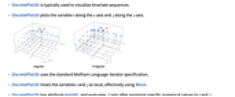
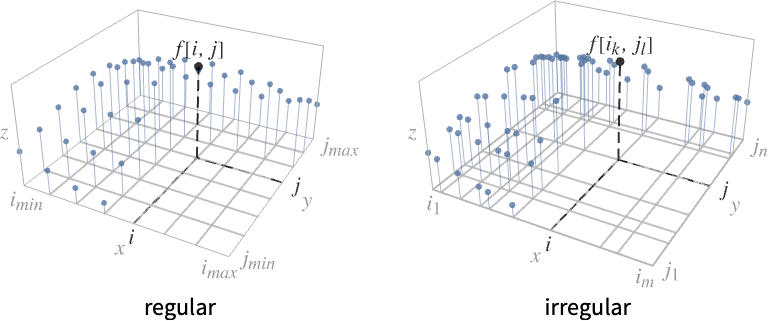
- DiscretePlot3D 通常用于可视化二元数列.
- DiscretePlot3D 沿
轴绘制 i 变量,沿
轴绘制 j 变量. - DiscretePlot3D 使用标准的 Wolfram 语言迭代器规范.
- DiscretePlot3D 视 i 和 j 为局部变量,实际上是在使用 Block.
- DiscretePlot3D 具有 HoldAll 属性,只有在对 i 和 j 赋以特定值以后才对 f 求值.
- 有时在对 i 和 j 赋以特定值以前,应用 Evaluate 符号式地对 f 求值可能会更有效.
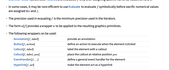
- 用于 f 求值的精度是迭代程序所用的最小精度i.
- 形式 w[f] 为所得图形基元提供一个包装 w.
- 可以用如下的包装:
-
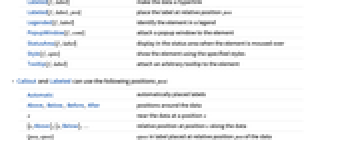
Annotation[f,label] 给出一个标注 Button[f,action] 定义一个单元被点击时要采取的动作 Callout[f,label] 用标注标记元素 Callout[f,label,pos] 把标注放在相关位置 pos EventHandler[f,…] 对单元定义一个通用的事件处理器 Hyperlink[f,uri] 将单元做成一个超链接 Labeled[f,label] 使数据成为超链接 Labeled[f,label,pos] 把标签放在相关位置 pos Legended[f,label] 标识图例中的数据 PopupWindow[f,cont] 对元素附加一个弹出窗口 StatusArea[f,label] 对单元附加一个弹出窗口 Style[f,opts] 鼠标滑过单元时在状态区域给予显示 Tooltip[f,label] 在单元上附加一个任意的工具提示 - Callout 和 Labeled 可用以下位置 pos:
-
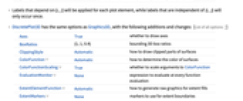
Automatic 自动放置标签 Above, Below, Before, After 数据周边的位置 x 靠近数据位置 x {s,Above},{s,Below},… 沿着数据位置 s 的相关位置 {pos,epos} 标签 epos 放在数据的相关位置 pos - 依赖于 {i,j} 的标签会应用于每个绘制元素,独立于 {i,j} 的标签仅出现一次.
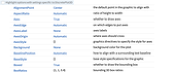
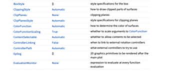
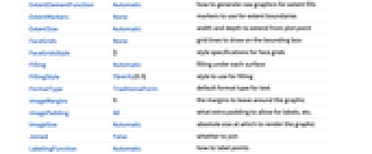
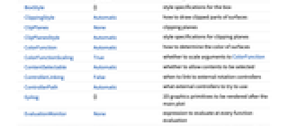
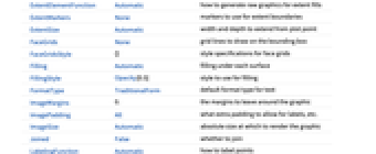
- DiscretePlot3D 具有与 Graphics3D 相同的选项,但有如下附加内容与变动: [所有选项的列表]
-
Axes True 是否绘制坐标轴 BoxRatios {1,1,0.4} 三维框界定比例 ClippingStyle Automatic 如何绘制曲面的裁剪部分 ColorFunction Automatic 如何确定曲面的颜色 ColorFunctionScaling True 是否根据 ColorFunction 缩放参变量 EvaluationMonitor None 在每个函数被求值时要求值的表达式 ExtentElementFunction Automatic 如何生成一个原始图以便作延伸填充 ExtentMarkers None 用于延伸边界的标符 ExtentSize Automatic 从绘制点作延伸的宽度和深度 Filling Automatic 每一个曲面下的填充 FillingStyle Opacity[0.5] 填充所用的样式 Joined False 是否连接 LabelingFunction Automatic 如何标签点 LabelingSize Automatic 标注和标签的最大尺寸 Method Automatic 所用的方法 PerformanceGoal $PerformanceGoal 性能上试图要优化的方面 PlotLegends None 序列的图例 PlotMarkers None 绘制点时使用的标记 PlotRange {Full,Full,Automatic} 所要包含的
或其它值的范围 PlotStyle Automatic 每个曲面的式样的图形指令 PlotTheme $PlotTheme 图形的全局主题 RegionFunction (True&) 如何确定是否要包括某个点 ScalingFunctions None 如何对单个坐标进行标度 WorkingPrecision MachinePrecision 内部计算所用的精度 - 传递给 ColorFunction 的参变量是
、
、
. - 通过设置 ExtentSize->{{sxl,sxr},{syl,syr}},每一个图形点周围将绘制一个水平平面,该平面沿
轴向左延伸到 sxl,向右延伸到 sxr ,沿
轴向左延伸到 syl,向右延伸到 syr. 设置 ExtentMarkers->{{mxl,mxr},{myl,myr}} 时,标符 mxl 和 mxr 将被用作沿
轴的左标符和右标符,标符 myl 和 myr 将被用作沿
轴的左标符和右标符. - ExtentElementFunction 的参量是单元之区域 {{xmin,xmax},{ymin,ymax},{zmin,zmax}} 及采样点 {xi,yi,zi}.
- 设置 ExtentSize->None 时, xmin 等于 xmax, ymin 等于 ymax. 设置 Filling->None 时, zmin 等于 zmax.
- PlotMarkers 的可能的设置包括:
-
None 绘制曲面时省略标记 "Point" 用 2D 点作为标记 "Sphere" 用 3D 球体作为标记 {"Point",s},{"Sphere",s} 指定标记的大小 s {spec1,spec2,…} 对表达式 expri 使用规范 speci - 标记的大小 s 可以是符号值,如 Tiny、Small、Medium 和 Large,或是图形宽度的缩放比例.
- ScalingFunctions 的可能设置包括:
-
sz 缩放 z 轴 {sx,sy} 缩放 x 和 y 轴 {sx,sy,sz} 缩放 x,y 和 z 轴 - 每个缩放函数 si 要么是字符串 "scale" 要么是 {g,g-1},其中 g-1 是 g 的倒数.
所有选项的列表
范例
打开所有单元 关闭所有单元基本范例 (3)
DiscretePlot3D[PDF[MultivariatePoissonDistribution[3, {1, 1}], {t, u}], {t, 0, 10}, {u, 0, 10}]DiscretePlot3D[PDF[MultivariatePoissonDistribution[3, {1, 1}], {t, u}], {t, 0, 10}, {u, 0, 10}, ExtentSize -> Full]DiscretePlot3D[{PDF[MultivariatePoissonDistribution[3, {1, 1}], {t, u}], PDF[MultivariatePoissonDistribution[5, {2, 2}], {t, u}]}, {t, 0, 10}, {u, 0, 10}, ExtentSize -> Full]范围 (12)
数据和布局 (4)
DiscretePlot3D[{Sin[t + u], Cos[t + u]}, {t, 0, 2Pi, Pi / 12}, {u, 0, 2Pi, Pi / 12}, ExtentSize -> Full]{DiscretePlot3D[{Sin[t + u], Cos[t + u]}, {t, 0, 2 * Pi, Pi / 6}, {u, 0, 2 * Pi, Pi / 6}, ExtentSize -> Full], DiscretePlot3D[{Sin[t + u], Style[Cos[t + u], Green]}, {t, 0, 2 * Pi, Pi / 6}, {u, 0, 2 * Pi, Pi / 6}, ExtentSize -> Full], DiscretePlot3D[Style[{Sin[t + u], Cos[t + u]}, Green], {t, 0, 2 * Pi, Pi / 6}, {u, 0, 2 * Pi, Pi / 6}, ExtentSize -> Full]}DiscretePlot3D[Style[{Sin[t + u], Style[Cos[t + u], Green]}, Red], {t, 0, 2 * Pi, Pi / 12}, {u, 0, 2 * Pi, Pi / 12}, ExtentSize -> Full]DiscretePlot3D[{Sin[t + u], Tooltip[Cos[t + u], "my data"]}, {t, 0, 2 * Pi, Pi / 12}, {u, 0, 2 * Pi, Pi / 12}, ExtentSize -> Full]使用 PopupWindow 来提供更多更深入的信息:
DiscretePlot3D[PopupWindow[PDF[MultivariatePoissonDistribution[3, {1, 1}], {t, u}], TraditionalForm[PDF[MultivariatePoissonDistribution[3, {1, 1}], {t, u}]]], {t, 0, 10}, {u, 0, 10}, ExtentSize -> Full]Button 可用来激活一个动作:
DiscretePlot3D[Evaluate@Table[With[{lambda = λ}, Button[PDF[
MultivariatePoissonDistribution[lambda, {1, 1}], {t, u}],
Speak[MultivariatePoissonDistribution[lambda, {1, 1}]]]], {λ, {1, 2, 3}}],
{t, 0, 10}, {u, 0, 10}, PlotRange -> All, ExtentSize -> Full]使用 ScalingFunctions 缩放轴:
DiscretePlot3D[LCM[x, y], {x, 20}, {y, 20}, ExtentSize -> Full, ScalingFunctions -> "Log"]标签和图例 (3)
DiscretePlot3D[Callout[GCD[x, y], If[x == y, x, None], Above], {x, Prime[Range[10]]}, {y, Prime[Range[10]]}]DiscretePlot3D[Tooltip[GCD[x, y], GCD[x, y]], {x, Prime[Range[10]]}, {y, Prime[Range[10]]}]使用 LabelingFunction 指定标签名称:
DiscretePlot3D[GCD[x, y], {x, 1, 5}, {y, 1, 5}, LabelingFunction -> (#1[[1]] &)]DiscretePlot3D[Callout[GCD[x, y], IntegerName@GCD[x, y]], {x, 1, 5}, {y, 1, 5}]样式及外观 (5)
用 ExtentSize 将一个点和一个区域相联系:
Table[DiscretePlot3D[PDF[MultivariatePoissonDistribution[3, {1, 1}], {t, u}], {t, 0, 10}, {u, 0, 10}, ExtentSize -> s, PlotLabel -> s], {s, {None, Full, Right, Scaled[0.5]}}]DiscretePlot3D[{Sin[t + u], Cos[t + u]}, {t, 0, 2 * Pi}, {u, 0, 2 * Pi}, PlotStyle -> {Red, Blue}, ExtentSize -> Full]使用 ColorData 提供的任何一个渐变配色方案:
{DiscretePlot3D[{Sin[t + u], Cos[t + u]}, {t, 0, 2 * Pi}, {u, 0, 2 * Pi}, ColorFunction -> "Pastel", ExtentSize -> Full], DiscretePlot3D[{Sin[t + u], Cos[t + u]}, {t, 0, 2 * Pi}, {u, 0, 2 * Pi}, ColorFunction -> Function[{x, y}, ColorData["NeonColors"][y]], ExtentSize -> Full]}Style 可以用来覆盖式样:
DiscretePlot3D[{Sin[t + u], Style[Cos[t + u], Red]}, {t, 0, 2 * Pi}, {u, 0, 2 * Pi}, PlotStyle -> Gray, ExtentSize -> Full]DiscretePlot3D[Exp[-x ^ 2 - y ^ 2], {x, -3, 3, 0.25}, {y, -3, 3, 0.25}, PlotMarkers -> "Sphere"]DiscretePlot3D[PDF[MultivariatePoissonDistribution[3, {1, 1}], {t, u}], {t, 10}, {u, 10}, ColorFunction -> "Rainbow", ExtentSize -> Full, ExtentMarkers -> "Tube"]DiscretePlot3D[PDF[MultivariatePoissonDistribution[3, {1, 1}], {t, u}], {t, 10}, {u, 10}, ExtentSize -> Full, ColorFunction -> "DarkRainbow", ExtentMarkers -> {{"Tube", None}, {"Tube", None}}]DiscretePlot3D[Mod[x, y], {x, 10}, {y, 10}, PlotTheme -> "Marketing"]选项 (90)
Axes (3)
默认情况下,为每个 DiscretePlot3D 绘制 Axes:
DiscretePlot3D[Mod[x, y], {x, 10}, {y, 10}, ExtentSize -> Full]DiscretePlot3D[Mod[x, y], {x, 10}, {y, 10}, ExtentSize -> Full, Axes -> False]{DiscretePlot3D[Mod[x, y], {x, 10}, {y, 10}, ExtentSize -> Full, Axes -> {True, False, False}], DiscretePlot3D[Mod[x, y], {x, 10}, {y, 10}, ExtentSize -> Full, Axes -> {False, True, False}], DiscretePlot3D[Mod[x, y], {x, 10}, {y, 10}, ExtentSize -> Full, Axes -> {False, False, True}]}AxesLabel (4)
DiscretePlot3D[Mod[x, y], {x, 10}, {y, 10}, ExtentSize -> Full]DiscretePlot3D[Mod[x, y], {x, 10}, {y, 10}, ExtentSize -> Full, AxesLabel -> "Mod[x,y]"]DiscretePlot3D[Mod[x, y], {x, 10}, {y, 10}, ExtentSize -> Full, AxesLabel -> {"x", "y", "Mod[x,y]"}]用 DiscretePlot3D 中指定的变量作为标签:
DiscretePlot3D[Mod[x, y], {x, 10}, {y, 10}, ExtentSize -> Full, AxesLabel -> Automatic]AxesOrigin (2)
AxesStyle (4)
DiscretePlot3D[Mod[x, y], {x, 10}, {y, 10}, ExtentSize -> Full, AxesStyle -> Red]DiscretePlot3D[Mod[x, y], {x, 10}, {y, 10}, ExtentSize -> Full, AxesStyle -> {{Thick, Brown}, {Thick, Blue}, {Thick, Green}}]DiscretePlot3D[Mod[x, y], {x, 10}, {y, 10}, ExtentSize -> Full, AxesStyle -> Green, TicksStyle -> StandardBlue]DiscretePlot3D[Mod[x, y], {x, 10}, {y, 10}, ExtentSize -> Full, AxesStyle -> Green, LabelStyle -> Black]ColorFunction (6)
Map[DiscretePlot3D[PDF[MultivariatePoissonDistribution[5, {2, 3}], {x, y}], {x, 0, 15}, {y, 0, 15}, ColorFunction -> Function[{x, y, z}, #], PlotLabel -> #]&, {Hue[x], Hue[y], Hue[z]}]Map[DiscretePlot3D[PDF[MultivariatePoissonDistribution[5, {2, 3}], {x, y}], {x, 0, 15}, {y, 0, 15}, Joined -> True, PlotRange -> All, ColorFunction -> Function[{x, y, z}, #], PlotLabel -> #]&, {Hue[x], Hue[y], Hue[z]}]Map[DiscretePlot3D[PDF[MultivariatePoissonDistribution[5, {2, 3}], {x, y}], {x, 0, 15}, {y, 0, 15}, ExtentSize -> Full, ColorFunction -> Function[{x, y, z}, #], PlotLabel -> #]&, {Hue[x], Hue[y], Hue[z]}]DiscretePlot3D[PDF[MultivariatePoissonDistribution[1, {1, 1}], {x, y}], {x, 0, 15}, {y, 0, 15}, ExtentSize -> Full, ColorFunction -> "Rainbow"]ColorFunction 优先于 PlotStyle:
DiscretePlot3D[PDF[MultivariatePoissonDistribution[5, {2, 3}], {x, y}], {x, 0, 15}, {y, 0, 15}, ColorFunction -> "Rainbow", PlotStyle -> Directive[Red, PointSize[Large]]]DiscretePlot3D[GCD[m, n], {m, 1, 20}, {n, 1, 20}, ExtentSize -> Full, ColorFunction -> Function[{x, y, z}, If[z == 1, Black, Hue[z / 20]]], ColorFunctionScaling -> False]ColorFunctionScaling (1)
EvaluationMonitor (1)
ExtentElementFunction (5)
为 ExtentElementFunction 获取一个内置设置的列表:
ChartElementData["DiscretePlot3D"]Table[DiscretePlot3D[PDF[MultivariatePoissonDistribution[1, {1, 1}], {x, y}], {x, 0, 8}, {y, 0, 8}, ExtentSize -> Full, ExtentElementFunction -> f], {f, {"Cone", "Cube", "Cylinder", "PlaneFadingCube"}}]Table[DiscretePlot3D[PDF[MultivariatePoissonDistribution[1, {1, 1}], {x, y}], {x, 0, 8}, {y, 0, 8}, ExtentSize -> Full, ExtentElementFunction -> f], {f, {"ProfileCube", "DoubleProfileCube", "SquareWaveCube", "TriangleWaveCube"}}]这个 ChartElementFunction 适合于显示全局标度:
Table[DiscretePlot3D[PDF[MultivariatePoissonDistribution[1, {1, 1}], {x, y}], {x, 0, 8}, {y, 0, 8}, ExtentSize -> Full, ExtentElementFunction -> f], {f, {"GradientScaleCube", "SegmentScaleCube"}}]编写一个客户指定的 ExtentElementFunction:
vase[{{xmin_, xmax_}, {ymin_, ymax_}, {zmin_, zmax_}}, ___] := {CapForm[None], Tube[
Table[{(xmin + xmax) / 2, (ymin + ymax) / 2, z}, {z, zmin, zmax, (zmax - zmin) / 15}],
Join[Sort[RandomReal[(xmax - xmin){0.1, 0.5}, 8], Less], Sort[RandomReal[(xmax - xmin){0.1, 0.5}, 8], Greater]]]}DiscretePlot3D[PDF[MultivariatePoissonDistribution[1, {1, 1}], {x, y}], {x, 0, 5}, {y, 0, 5}, ExtentSize -> Full, ExtentElementFunction -> vase, PlotRange -> {0, 0.1}]一个内置的函数可以含有某些选项;可用 面板 ▶ 图表元素方案 对它们进行设置:
ChartElementData["ProfileCube", "Options"]Table[DiscretePlot3D[PDF[MultivariatePoissonDistribution[1, {1, 1}], {x, y}], {x, 0, 5}, {y, 0, 5}, ExtentSize -> Full, ExtentElementFunction -> ChartElementData["ProfileCube", "Profile" -> p, "TaperRatio" -> r]], {p, {0.1, 1, 5}}, {r, {0, 0.5, 1}}]ExtentMarkers (4)
DiscretePlot3D[LCM[m, n], {m, 6}, {n, 6}, ExtentSize -> Full, ExtentMarkers -> None, PlotStyle -> EdgeForm[]]DiscretePlot3D[LCM[m, n], {m, 6}, {n, 6}, ExtentSize -> Full, ExtentMarkers -> {"Line", 5}, PlotStyle -> EdgeForm[]]Table[DiscretePlot3D[LCM[m, n], {m, 5}, {n, 5}, ExtentSize -> Full, ExtentMarkers -> {"Tube", size}], {size, {Tiny, Small, Medium, Large}}]DiscretePlot3D[LCM[m, n], {m, 5}, {n, 5}, ExtentSize -> Full, ExtentMarkers -> {{"Tube", None}, {"Tube", None}}]ExtentSize (6)
DiscretePlot3D[LCM[m, n], {m, 5}, {n, 5}, ExtentSize -> None]DiscretePlot3D[LCM[m, n], {m, 5}, {n, 5}, ExtentSize -> Full]DiscretePlot3D[LCM[m, n], {m, {1, 2, 3, 5, 8, 13}}, {n, {1, 2, 3, 5, 8, 13}}, ExtentSize -> Full]DiscretePlot3D[LCM[m, n], {m, 5}, {n, 5}, ExtentSize -> 0.5]DiscretePlot3D[LCM[m, n], {m, {1, 2, 3, 5, 8, 13}}, {n, {1, 2, 3, 5, 8, 13}}, ExtentSize -> 0.5]DiscretePlot3D[LCM[m, n], {m, 5}, {n, 5}, ExtentSize -> Scaled[0.75]]DiscretePlot3D[LCM[m, n], {m, {1, 2, 3, 5, 8, 13}}, {n, {1, 2, 3, 5, 8, 13}}, ExtentSize -> Scaled[0.75]]DiscretePlot3D[LCM[m, n], {m, 5}, {n, 5}, ExtentSize -> All]DiscretePlot3D[LCM[m, n], {m, {1, 2, 3, 5, 8, 13}}, {n, {1, 2, 3, 5, 8, 13}}, ExtentSize -> All]Table[DiscretePlot3D[LCM[m, n], {m, 5}, {n, 5}, ExtentSize -> es, PlotLabel -> es, PlotMarkers -> {"Sphere", Large}], {es, {{{None, Full}, {None, Full}}, {{Full, None}, {Full, None}}}}]Filling (3)
DiscretePlot3D 填充到
:
Table[DiscretePlot3D[Mod[m, n], {m, 15}, {n, 15}, Evaluate[opt]], {opt, {Joined -> False, Joined -> True, ExtentSize -> Full}}]Table[DiscretePlot3D[Mod[m, n], {m, 15}, {n, 15}, Filling -> None, Evaluate[opt]], {opt, {Joined -> False, Joined -> True, ExtentSize -> Full}}]Table[DiscretePlot3D[Mod[m, n] - Mod[n, m], {m, 15}, {n, 15}, Filling -> fill, PlotLabel -> fill], {fill, {Bottom, Top, Axis, -20}}]FillingStyle (3)
Table[DiscretePlot3D[Mod[m, n] - Mod[n, m], {m, 15}, {n, 15}, Filling -> Bottom, FillingStyle -> fs], {fs, {Opacity[1], Red, Dashed, Thick}}]Table[DiscretePlot3D[Mod[m, n] - Mod[n, m], {m, 15}, {n, 15}, ExtentSize -> Full, Filling -> Bottom, FillingStyle -> fs], {fs, {Opacity[1], Red}}]Table[DiscretePlot3D[Mod[m, n] - Mod[n, m], {m, 15}, {n, 15}, ExtentSize -> es, Filling -> Axis, FillingStyle -> {Red, Blue}], {es, {None, Full}}]Table[DiscretePlot3D[Mod[m, n] - Mod[n, m], {m, 15}, {n, 15}, ExtentSize -> es, Filling -> Axis, FillingStyle -> {Red, None}], {es, {None, Full}}]ImageSize (7)
使用已命名尺寸,如 Tiny、Small、Medium 和 Large:
{DiscretePlot3D[Mod[x, y], {x, 10}, {y, 10}, ExtentSize -> Full, ImageSize -> Tiny], DiscretePlot3D[Mod[x, y], {x, 10}, {y, 10}, ExtentSize -> Full, ImageSize -> Small]}{DiscretePlot3D[Mod[x, y], {x, 10}, {y, 10}, ExtentSize -> Full, ImageSize -> 150], DiscretePlot3D[Mod[x, y], {x, 10}, {y, 10}, ExtentSize -> Full, AspectRatio -> 1.5, ImageSize -> 150]}{DiscretePlot3D[Mod[x, y], {x, 10}, {y, 10}, ExtentSize -> Full, ImageSize -> {Automatic, 150}], DiscretePlot3D[Mod[x, y], {x, 10}, {y, 10}, ExtentSize -> Full, AspectRatio -> 2, ImageSize -> {Automatic, 150}]}{DiscretePlot3D[Mod[x, y], {x, 10}, {y, 10}, ExtentSize -> Full, ImageSize -> UpTo[200]], DiscretePlot3D[Mod[x, y], {x, 10}, {y, 10}, ExtentSize -> Full, AspectRatio -> 2, ImageSize -> UpTo[200]]}DiscretePlot3D[Mod[x, y], {x, 10}, {y, 10}, ExtentSize -> Full, ImageSize -> {200, 250}, Background -> StandardGray]设置 AspectRatioFull 将填充可用空间:
DiscretePlot3D[Mod[x, y], {x, 10}, {y, 10}, ExtentSize -> Full, AspectRatio -> Full, ImageSize -> {200, 250}, Background -> StandardGray]{DiscretePlot3D[Mod[x, y], {x, 10}, {y, 10}, ExtentSize -> Full, ImageSize -> {UpTo[150], UpTo[100]}], DiscretePlot3D[Mod[x, y], {x, 10}, {y, 10}, ExtentSize -> Full, AspectRatio -> 2, ImageSize -> {UpTo[150], UpTo[100]}]}Framed[Pane[DiscretePlot3D[Mod[x, y], {x, 10}, {y, 10}, ExtentSize -> Full, ImageSize -> Full, Background -> StandardGray], {200, 100}]]Framed[Pane[DiscretePlot3D[Mod[x, y], {x, 10}, {y, 10}, ExtentSize -> Full, AspectRatio -> Full, ImageSize -> {Scaled[0.5], Scaled[0.5]}, Background -> StandardGray], {250, 250}]]Joined (2)
DiscretePlot3D[PDF[MultivariatePoissonDistribution[5, {2, 3}], {x, y}], {x, 0, 15}, {y, 0, 15}, Joined -> True]DiscretePlot3D[PDF[MultivariatePoissonDistribution[5, {2, 3}], {x, y}], {x, 0, 15}, {y, 0, 15}, Joined -> True, ExtentSize -> Full]LabelingFunction (4)
DiscretePlot3D[GCD[x, y], {x, 1, 5}, {y, 1, 5}, LabelingFunction -> Above]DiscretePlot3D[GCD[x, y], {x, 1, 5}, {y, 1, 5}, LabelingFunction -> Tooltip]DiscretePlot3D[GCD[x, y], {x, 1, 5}, {y, 1, 5}, LabelingFunction -> Callout[Automatic, Automatic]]DiscretePlot3D[GCD[x, y], {x, 1, 5}, {y, 1, 5}, LabelingFunction -> (#1&)]DiscretePlot3D[GCD[x, y], {x, 1, 5}, {y, 1, 5}, LabelingFunction -> (#2&)]LabelingSize (1)
DiscretePlot3D[Callout[GCD[x, y], IntegerName[x]], {x, 500, 505}, {y, 500, 505}, ImageSize -> Medium, LabelingSize -> 30]DiscretePlot3D[Callout[x + y, IntegerName[x + y]], {x, 0, 10}, {y, 0, 10}, ImageSize -> Medium, LabelingSize -> Full]PlotLegends (6)
DiscretePlot3D[{Sin[x + y], Cos[x + y]}, {x, 20}, {y, 20}, ExtentSize -> Full, PlotLegends -> Automatic]DiscretePlot3D[{x, y}, {x, 20}, {y, 20}, ExtentSize -> Full, PlotLegends -> {"label1", "label2"}]DiscretePlot3D[{Sin[x + y], Sin[x - y]}, {x, 20}, {y, 20}, ExtentSize -> Full, PlotLegends -> "Expressions"]PlotLegends 自动选择 PlotStyle 值:
DiscretePlot3D[{Sin[(x + y) ^ 2], Sin[(x - y) ^ 2]}, {x, 0, 2, 0.2}, {y, 0, 2, 0.2}, ExtentSize -> Full, PlotStyle -> {Red, Blue}, PlotLegends -> "Expressions"]使用 Placed 控制图例位置:
Table[DiscretePlot3D[{Sin[(x + y)], Sin[(x - y)]}, {x, 0, 2, 0.2}, {y, 0, 2, 0.2}, ExtentSize -> Full, PlotStyle -> {Orange, Blue}, PlotLegends -> Placed["Expressions", pos]], {pos, {Above, Below}}]使用 SwatchLegend 改变图例外观:
DiscretePlot3D[{Sin[(x + y) ^ 2], Sin[(x - y) ^ 2]}, {x, 0, 2, 0.2}, {y, 0, 2, 0.2}, ExtentSize -> Full, PlotStyle -> {Red, Blue}, PlotLegends -> SwatchLegend["Expressions", LegendLabel -> "label", LegendFunction -> (Framed[#, RoundingRadius -> 5]&)]]PlotMarkers (4)
Table[DiscretePlot3D[PDF[MultivariatePoissonDistribution[5, {2, 3}], {x, y}], {x, 0, 15}, {y, 0, 15}, PlotMarkers -> {Automatic, s}], {s, {Tiny, Small, Medium, Large}}]{DiscretePlot3D[PDF[MultivariatePoissonDistribution[5, {2, 3}], {x, y}], {x, 0, 15}, {y, 0, 15}, Joined -> True], DiscretePlot3D[PDF[MultivariatePoissonDistribution[5, {2, 3}], {x, y}], {x, 0, 15}, {y, 0, 15}, ExtentSize -> Full]}{DiscretePlot3D[PDF[MultivariatePoissonDistribution[5, {2, 3}], {x, y}], {x, 0, 15}, {y, 0, 15}, Joined -> True, PlotMarkers -> "Point", PlotStyle -> FaceForm[Lighter[Blue, 0.5]]], DiscretePlot3D[PDF[MultivariatePoissonDistribution[5, {2, 3}], {x, y}], {x, 0, 15}, {y, 0, 15}, ExtentSize -> Full, PlotMarkers -> "Point"]}{DiscretePlot3D[PDF[MultivariatePoissonDistribution[5, {2, 3}], {x, y}], {x, 0, 15}, {y, 0, 15}, PlotMarkers -> "Sphere"], DiscretePlot3D[PDF[MultivariatePoissonDistribution[5, {2, 3}], {x, y}], {x, 0, 15}, {y, 0, 15}, ExtentSize -> Full, PlotMarkers -> "Sphere"]}Table[DiscretePlot3D[PDF[MultivariatePoissonDistribution[5, {2, 3}], {x, y}], {x, 0, 15}, {y, 0, 15}, PlotMarkers -> {"Sphere", s}], {s, {Tiny, Small, Medium, Large}}]PlotStyle (7)
Table[DiscretePlot3D[PDF[MultivariatePoissonDistribution[5, {2, 3}], {x, y}], {x, 0, 15}, {y, 0, 15}, PlotStyle -> ps], {ps, {Red, PointSize[0.025], Darker[Green], Directive[Red, PointSize[Small]]}}]DiscretePlot3D[Evaluate[Table[PDF[MultivariatePoissonDistribution[2k, {k, 3k}], {x, y}], {k, 3}]], {x, 20}, {y, 20}, ExtentSize -> Full]DiscretePlot3D[Evaluate[Table[PDF[MultivariatePoissonDistribution[2k, {k, 3k}], {x, y}], {k, 3}]], {x, 20}, {y, 20}, ExtentSize -> Full, PlotStyle -> {Red, Orange, Blue}]PlotStyle 适用于点、线和曲面:
DiscretePlot3D[PDF[MultivariatePoissonDistribution[5, {2, 3}], {x, y}], {x, 0, 15}, {y, 0, 15}, PlotStyle -> Red]DiscretePlot3D[PDF[MultivariatePoissonDistribution[5, {2, 3}], {x, y}], {x, 0, 15}, {y, 0, 15}, ExtentSize -> Full, PlotStyle -> Directive[Orange, EdgeForm[Blue]]]PlotStyle 可以和 ColorFunction 结合使用:
DiscretePlot3D[PDF[MultivariatePoissonDistribution[5, {2, 3}], {x, y}], {x, 0, 15}, {y, 0, 15}, PlotStyle -> PointSize[Medium], ColorFunction -> Function[{x, y, z}, Hue[z]]]PlotStyle 可以和 FillingStyle 结合使用:
DiscretePlot3D[PDF[MultivariatePoissonDistribution[5, {2, 3}], {x, y}], {x, 0, 15}, {y, 0, 15}, PlotStyle -> Red, FillingStyle -> Opacity[1]]FillingStyle 默认时使用和 PlotStyle 相同的式样,包括透明度:
DiscretePlot3D[PDF[MultivariatePoissonDistribution[5, {2, 3}], {x, y}], {x, 0, 15}, {y, 0, 15}, PlotStyle -> Red]PlotTheme (4)
DiscretePlot3D[{CDF[MultivariatePoissonDistribution[3, {1, 1}], {t, u}], SurvivalFunction[MultivariatePoissonDistribution[3, {1, 1}], {t, u}]}, {t, 10}, {u, 10}, PlotTheme -> "Business"]DiscretePlot3D[{CDF[MultivariatePoissonDistribution[3, {1, 1}], {t, u}], SurvivalFunction[MultivariatePoissonDistribution[3, {1, 1}], {t, u}]}, {t, 10}, {u, 10}, PlotTheme -> "Business", PlotStyle -> {Red, Blue}]DiscretePlot3D[GCD[m, n], {m, 15}, {n, 15}, PlotTheme -> "Marketing"]DiscretePlot3D[GCD[m, n], {m, 15}, {n, 15}, PlotTheme -> "Marketing", Ticks -> None]RegionFunction (4)
DiscretePlot3D[GCD[m, n], {m, 25}, {n, 25}, RegionFunction -> Function[{m, n, z}, m ≤ n]]DiscretePlot3D[GCD[m, n], {m, 5}, {n, 5}, ExtentSize -> Full, RegionFunction -> Function[{m, n, z}, m <= n], PlotMarkers -> "Sphere"]DiscretePlot3D[GCD[m, n], {m, 25}, {n, 25}, RegionFunction -> Function[{m, n, z}, Mod[m + n, 10] ≤ 7]]DiscretePlot3D[GCD[m, n], {m, 25}, {n, 25}, RegionFunction -> Function[{m, n, z}, m ^ 2 + n ^ 2 ≤ 625 && m + n ≥ 25]]ScalingFunctions (9)
DiscretePlot3D[Max[x, y], {x, 0, 10, .5}, {y, 0, 10, .5}, ExtentSize -> Full]DiscretePlot3D[Max[x, y], {x, 1, 10, .5}, {y, 1, 10, .5}, ExtentSize -> Full, ScalingFunctions -> "Log"]DiscretePlot3D[Max[x, y], {x, 0, 10, .5}, {y, 0, 10, .5}, ExtentSize -> Full, ScalingFunctions -> {None, "Reverse"}]DiscretePlot3D[Max[x, y], {x, 1, 10, .5}, {y, 1, 10, .5}, ExtentSize -> Full, ScalingFunctions -> {None, "Reciprocal"}]DiscretePlot3D[Max[x, y], {x, 0, 10, .5}, {y, 0, 10, .5}, ExtentSize -> Full, ScalingFunctions -> {"Reverse", "Log"}]DiscretePlot3D[Max[x, y], {x, 0, 10, .5}, {y, 0, 10, .5}, ExtentSize -> Full, ScalingFunctions -> {"Reverse", None}]DiscretePlot3D[Max[x, y], {x, 0, 10, .5}, {y, 0, 10, .5}, ExtentSize -> Full, ScalingFunctions -> {None, {-Log[#]&, Exp[-#]&}}]DiscretePlot3D[u + t ^ 2, {t, 0.01, 50}, {u, 0, 10}, ExtentSize -> Full, ScalingFunctions -> {"Log", None}, Ticks -> {2 ^ Range[10], Automatic, Automatic}, FaceGrids -> All]PlotRange 是自动标度的:
DiscretePlot3D[LCM[m, n], {m, 50}, {n, 50}, ExtentSize -> Full, ScalingFunctions -> "Log", PlotRange -> {100, 1000}]应用 (2)
Table[DiscretePlot3D[PDF[MultivariatePoissonDistribution[μ, {2, 3}], {x, y}], {x, 0, 15}, {y, 0, 15}, ExtentSize -> 0.5, PlotLabel -> Row[{"μ = ", μ}]], {μ, {1, 5}}]Table[DiscretePlot3D[CDF[MultivariatePoissonDistribution[μ, {2, 3}], {x, y}], {x, 0, 15}, {y, 0, 15}, PlotStyle -> Purple, ExtentSize -> Right, PlotLabel -> Row[{"μ = ", μ}]], {μ, {1, 5}}]Table[DiscretePlot3D[SurvivalFunction[MultivariatePoissonDistribution[μ, {2, 3}], {x, y}], {x, 0, 15}, {y, 0, 15}, PlotStyle -> Orange, ExtentSize -> Right, PlotLabel -> Row[{"μ = ", μ}]], {μ, {1, 5}}]plot = Plot3D[PDF[BinormalDistribution[0.5], {x, y}], {x, -2, 2}, {y, -2, 2}, PlotStyle -> Directive[Opacity[0.4], Yellow], RegionFunction -> (# < 0 || #2 > 0&)]riemann = DiscretePlot3D[PDF[BinormalDistribution[0.5], {x, y}], {x, -2, 2, 0.5}, {y, -2, 2, 0.5}, ExtentSize -> Full, RegionFunction -> (# < 0 || #2 > 0&)]Show[plot, riemann]属性和关系 (4)
Plot3D 生成连续的曲面:
Plot3D[PDF[BinormalDistribution[0.5], {x, y}], {x, -2, 2}, {y, -2, 2}]用 ListPointPlot3D 绘制数值的列表的图形::
{ListPointPlot3D[Table[Table[x + y, {x, 10}], {y, 10}]], DiscretePlot3D[x + y, {x, 10}, {y, 10}]}用 BarChart3D 显示数值的列表的条形图:
{BarChart3D[Table[Table[x + y, {x, 10}], {y, 10}], ChartLayout -> "Grid"], DiscretePlot3D[x + y, {x, 10}, {y, 10}, ExtentSize -> Full]}用 DiscretePlot 绘制离散单变量函数的图形:
DiscretePlot[PDF[PoissonDistribution[4], x], {x, 0, 10}, ExtentSize -> Scaled[0.5]]文本
Wolfram Research (2010),DiscretePlot3D,Wolfram 语言函数,https://reference.wolfram.com/language/ref/DiscretePlot3D.html (更新于 2019 年).
CMS
Wolfram 语言. 2010. "DiscretePlot3D." Wolfram 语言与系统参考资料中心. Wolfram Research. 最新版本 2019. https://reference.wolfram.com/language/ref/DiscretePlot3D.html.
APA
Wolfram 语言. (2010). DiscretePlot3D. Wolfram 语言与系统参考资料中心. 追溯自 https://reference.wolfram.com/language/ref/DiscretePlot3D.html 年
BibTeX
@misc{reference.wolfram_2026_discreteplot3d, author="Wolfram Research", title="{DiscretePlot3D}", year="2019", howpublished="\url{https://reference.wolfram.com/language/ref/DiscretePlot3D.html}", note=[Accessed: 13-September-2026]}
BibLaTeX
@online{reference.wolfram_2026_discreteplot3d, organization={Wolfram Research}, title={DiscretePlot3D}, year={2019}, url={https://reference.wolfram.com/language/ref/DiscretePlot3D.html}, note=[Accessed: 13-September-2026]}