ComplexListPlot[{z1,z2,…}]
複素数 z1, z2, …を複素平面上の点としてプロットする.
ComplexListPlot[{data1,data2,…}]
全 dataiからのデータをプロットする.
ComplexListPlot[{…,w[datai,…],…}]
記号ラッパー w で特徴が定義された
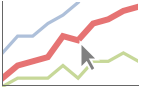
をプロットする.
ComplexListPlot
ComplexListPlot[{z1,z2,…}]
複素数 z1, z2, …を複素平面上の点としてプロットする.
ComplexListPlot[{data1,data2,…}]
全 dataiからのデータをプロットする.
ComplexListPlot[{…,w[datai,…],…}]
記号ラッパー w で特徴が定義された
をプロットする.
詳細とオプション
- dataiは,次の形式と解釈を持つ.
-
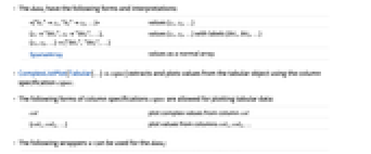
<|"k1"z1,"k2"z2,…|> 値{z1,z2,…} {z1"lbl1",z2"lbl2",…}, {z1,z2,…}{"lbl1","lbl2",…} ラベル{lbl1,lbl2,…}付きの値{z1,z2,…} SparseArray 通常の配列としての値 - ComplexListPlot[objcspec]は,列指定 cspec を用いて,Tabular,TimeSeriesまたはEventSeriesオブジェクト obj から値を抽出してプロットする.
- 次は,表形式データのプロットに使用可能な列指定 cspec の形式である.
-
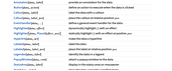
col 列 col からの複素数値をプロットする {col1,col2,…} 列 col1, col2, …からの値をプロットする - dataiには次のラッパー w を使うことができる.
-
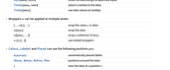
Annotation[datai,label] データの注釈を与える Button[datai,action] データがクリックされたときのアクションを定義する Callout[datai,label] データにコールアウトでラベルを付ける Callout[datai,label,pos] 相対位置 pos にコールアウトを置く EventHandler[datai,…] データの一般的なイベントハンドラを定義する Highlighted[datai,effect] 効果を使って fiを動的にハイライトする Highlighted[datai,Placed[effect,pos]] 位置 pos で効果を使って fiを静的にハイライトする Hyperlink[datai,uri] データをハイパーリンクにする Labeled[datai,label] データにラベルを付ける Labeled[datai,label,pos] 相対位置 pos にラベルを置く Legended[datai,label] データを凡例の中で識別する PopupWindow[datai,cont] データにポップアップウィンドウを付ける StatusArea[datai,label] マウスオーバーのときにステータスエリアに表示する Style[datai,styles] データを指定されたスタイルで表示する Tooltip[datai,label] データにツールチップを付ける Tooltip[datai] データの値をツールチップとして使う - ラッパー w は複数レベルで適用することができる.
-
{…,w[zi],…} データの値 ziをラップする w[datai] データをラップする w[{data1,…}] dataiの集合をラップする w1[w2[…]] ネストしたラッパーを使う - Callout,Labeled,Placedには次の位置 pos を使うことができる.
-
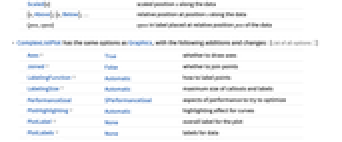
Automatic 自動的に置かれたラベル Above, Below, Before, After データ周囲の位置 x 位置 x のデータの近く Scaled[s] データに沿った,スケールされた位置 s {s,Above},{s,Below},… データに沿った,位置 s の相対位置 {pos,epos} データと相対的な位置 pos に置かれたラベルの中の epos - ComplexListPlotにはGraphicsと同じオプションに以下の追加・変更を加えたものが使える. [全オプションのリスト]
-
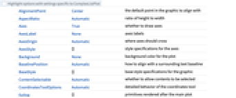
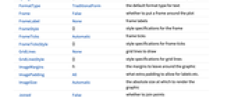
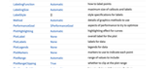
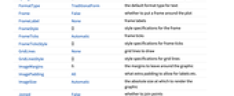
Axes True 軸を描くかどうか Joined False 点を繋ぐかどうか LabelingFunction Automatic 点にどのようにラベルを付けるか LabelingSize Automatic コールアウトとラベルの最大サイズ PerformanceGoal $PerformanceGoal パフォーマンスのどの面について最適化するか PlotHighlighting Automatic 曲線のハイライト効果 PlotLabel None プロットの全体的なラベル PlotLabels None データのラベル PlotLegends None データの凡例 PlotMarkers None 各点を示すために使うマーカー PlotRange Automatic 含める値の範囲 PlotRangeClipping True プロット範囲で切り取るかどうか PlotStyle Automatic 点のスタイルを決定するグラフィックス指示子 PlotTheme $PlotTheme プロットの全体的なテーマ PolarAxes False 極座標軸を描くかどうか PolarAxesOrigin Automatic どこに極座標軸を描くか PolarGridLines None 描く極格子線 PolarTicks Automatic 極座標軸の目盛 ScalingFunctions None 個々の座標をどのようにスケールするか - LabelingFunction->f は各点に f[value,index,lbls]で与えられるラベルを付けるように指定する.ただし,value は点に関連付けられた値,index は data 内の位置,lbls は関連するラベルのリストである.
- 次は,PlotLegendsのよく使われる設定である.
-
None 凡例は使わない Automatic 凡例を自動的に決定する {lbl1,lbl2,…} lbl1, lbl2, …を凡例として使う Placed[lspec,…] 凡例の置き方を指定する - PlotStylesty は,各曲線に使用するスタイルを指定する.可能な設定には次が含まれる.
-
{sty1,sty2,…} データ集合に対するスタイルの列 <|"key"val,…|> データの異なるレベルに対するスタイル要素 - 使用可能なキーは次の通りである.
-
"Base" すべての dataiに対する全体的なスタイル "Lists" dataiごとのスタイル styiのリスト - ColorData["DefaultPlotColors"]は,PlotStyleによって使用されるデフォルトの色の並びを与える.
- MeshFunctions内の関数に与えられる偏角は,x, y, θ, r である.θ と r は ziの偏角と半径である.ColorFunction内の関数には,デフォルトで,これらの偏角のスケールされたバージョンが与えられる.
- 次は,HighlightedとPlotHighlightingに使用可能なハイライト効果である.
-
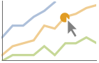
style 指定されたデータをハイライトする 
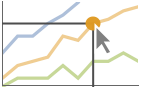
"Ball" データ上の指定された点をハイライトしてラベルを付ける 

"Dropline" データ上の指定された点を軸までのドロップラインでハイライトしてラベルを付ける 
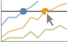
"XSlice" 垂直スライスに沿ったすべての点をハイライトしてラベルを付ける 
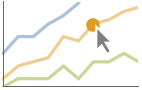
"YSlice" 水平スライスに沿ったすべての点をハイライトしてラベルを付ける 
Placed[effect,pos] 指定の位置 pos を静的にハイライトする - ハイライトの位置指定 pos には次がある.
-
x, {x} {x,y}における効果.y は自動的に選択される {x,y} {x,y}における効果 {pos1,pos2,…} 複数の位置 posi - ScalingFunctions->"scale"は ziの絶対値をスケールする.ScalingFunctions{"scalex","scaley"}はそれぞれ実部成分と虚部成分をスケールする.
全オプションのリスト
例題
すべて開く すべて閉じる例 (4)

ComplexListPlot[{-2 - 2 I, -1 - I, 0, 1 + I, 2 + 2 I}]ComplexListPlot[{RandomComplex[{0, 1 + I}, 100], RandomComplex[{-2 - 2I, 2 + 2I}, 100]}]data = Table[a t Exp[2 π I t], {a, 2, 4}, {t, 0, 1, 0.02}];
ComplexListPlot[data, PlotLegends -> {"a=2", "a=3", "a=4"}]ComplexListPlot[Callout[#, #]& /@ Table[E^π I k / 4, {k, 1, 8}]]スコープ (39)
データ (7)
ComplexListPlot[Sin[Range[40] + 2I]]ComplexListPlot[{Sin[Range[40] + 2I], Cos[Range[40] + 2I]}]ComplexListPlot[{1 + I, 2 + 2I, Missing["NotAvailable"], 4 + 4I, None, 6 + 6I, ""}]MaxPlotPointsを使って使用する点の数を制限する:
data = Table[Exp[2Pi I RandomReal[]], {n, 200}];
Table[ComplexListPlot[data, MaxPlotPoints -> mp], {mp, {Infinity, 100, 50}}]PlotRangeは自動的に選択される:
{ComplexListPlot[{0, 1 + I, 2 + 2I, 3 + 3I, 4 + 20I, 5 + 5I, 20 + 6I}],
ComplexListPlot[{0, 1 + I, 2 + 2I, 3 + 3I, 4 + 20I, 5 + 5I, 20 + 6I}, PlotRange -> All]}PlotRangeを使って関心領域に焦点を当てる:
{ComplexListPlot[{0, 1 + I, 2 + 2I, 3 + 3I, 4 + 100I, 5 + 5I, 20 + 6I}],
ComplexListPlot[{0, 1 + I, 2 + 2I, 3 + 3I, 4 + 100I, 5 + 5I, 20 + 6I}, PlotRange -> {0, 7 + 7I}]}ScalingFunctionsを使って軸をスケールする:
ComplexListPlot[Table[10^k + 2^kI, {k, -2, 5}], ScalingFunctions -> {"Log10", "Log2"}]表形式データ (1)
ニュートン法でランダムな開始シードで
を解いた結果の表形式データを入手する:
tab = Tabular[IconizedObject[«data»], {"seed", "solution", "basin"}]ComplexListPlot[tab -> "seed", PlotStyle -> AbsolutePointSize[2]]PivotToColumnsを使って各引込み領域について列を生成する:
pivot = PivotToColumns[tab, "basin" -> "seed"]ComplexListPlot[pivot -> {Key[1], Key[2], Key[3]}, PlotStyle -> AbsolutePointSize[2]]特殊データ (4)
ComplexListPlot[{1 + I -> "a", 2 + 2I -> "b", 3 + 3I -> "c", 4 + 4I -> "d", 5 + 3I -> "e", 6 + 2I -> "f", 7 + I -> "g"}]
ComplexListPlot[{1 + I, 2 + 2 I, 3 + 3 I, 4 + 4 I, 5 + 3 I, 6 + 2 I, 7 + I} -> {"a", "b", "c", "d", "e", "f", "g"}]ComplexListPlot[{1 + I, 2 + 2 I, 3 + 3 I, 4 + 4 I, 5 + 3 I, 6 + 2 I, 7 + I} -> {"a", "b", "c", "d", "e", "f", "g"}, LabelingFunction -> Above]Association中の数値は
座標として使われる:
ComplexListPlot[<|"a" -> 2 + I, "b" -> 3 - I, "c" -> 5 + 2I, "d" -> 7, "e" -> 11 + 2I, "f" -> 13 - 3I|>]SparseArray中のデータをプロットする:
ComplexListPlot[SparseArray[RandomComplex[{0, 1 + I}, 25]]]ラッパー (6)
個々のデータ,データ集合,あるいはデータ集合の集合にラッパーを使う:
{ComplexListPlot[{{1 + I, Style[3 + 2I, Red], 6 + 3I}, {1 + 4I, 3 + 5I, 6 + 6I}}, PlotStyle -> PointSize[0.05]],
ComplexListPlot[{Style[{1 + I, 3 + 2I, 6 + 3I}, Red], {1 + 4I, 3 + 5I, 6 + 6I}}, PlotStyle -> PointSize[0.05]],
ComplexListPlot[Style[{{1 + I, 3 + 2I, 6 + 3I}, {1 + 4I, 3 + 5I, 6 + 6I}}, Red], PlotStyle -> PointSize[0.05]]}{ComplexListPlot[{{1 + I, Style[3 + 2I, Red], 6 + 3I}, {1 + 4I, 3 + 5I, 6 + 6I}}, PlotStyle -> PointSize[0.05]],
ComplexListPlot[{Style[{1 + I, Style[3 + 2I, Red], 6 + 3I}, Green], {1 + 4I, 3 + 5I, 6 + 6I}}, PlotStyle -> PointSize[0.05]],
ComplexListPlot[Style[{Style[{1 + I, Style[3 + 2I, Red], 6 + 3I}, Green], {1 + 4I, 3 + 5I, 6 + 6I}}, Blue], PlotStyle -> PointSize[0.05]]}ComplexListPlot[Tooltip[Table[k + Sqrt[k]I, {k, 10}], "square roots"]]ComplexListPlot[Table[Labeled[RandomComplex[{0, 1 + I}], i], {i, 20}], PlotStyle -> PointSize[Medium], ImageSize -> 300]PopupWindowを使って固有値をクリックし,対応する固有ベクトルを見る:
{evalues, evecs} = Eigensystem[RandomComplex[{-1 - I, 1 + I}, {4, 4}]];
ComplexListPlot[PopupWindow@@@Transpose[{evalues, evecs}], PlotStyle -> PointSize[0.04]]Buttonを使って任意のアクションを引き起こすことができる:
evalues = Eigenvalues[RandomComplex[{-1 - I, 1 + I}, {8, 8}]];
ComplexListPlot[Button[#, Speak[#]]& /@ evalues, PlotStyle -> PointSize[0.02]]ラベル付けと凡例 (15)
ComplexListPlot[Table[Labeled[RandomComplex[{0, 1 + I}], i], {i, 20}]]Table[ComplexListPlot[Table[Labeled[RandomComplex[{0, 1 + I}], i, p], {i, 20}], PlotLabel -> p], {p, {Above, Below, Before, After}}]Labeledでデータにラベルを付ける:
ComplexListPlot[{
Labeled[NestList[(0.9 + 0.1I)#&, 1 + I, 30], 0.1], Labeled[NestList[(0.9 + 0.2I)#&, 1 + I, 30], 0.2]
}]PlotLabelsでデータにラベルを付ける:
ComplexListPlot[{
NestList[(0.9 + 0.1I)#&, 1 + I, 30], NestList[(0.9 + 0.2I)#&, 1 + I, 30]
}, PlotLabels -> {0.1, 0.2}]ComplexListPlot[{
Labeled[NestList[(0.9 + 0.1I)#&, 1 + I, 30], 0.1, 0.1], Labeled[NestList[(0.9 + 0.2I)#&, 1 + I, 30], 0.2, 0.3]
}]ComplexListPlot[{
Labeled[NestList[(0.9 + 0.1I)#&, 1 + I, 30], 0.1, Scaled[0.1]], Labeled[NestList[(0.9 + 0.2I)#&, 1 + I, 30], 0.2, Scaled[0.1]]
}]ComplexListPlot[{
Labeled[NestList[(0.9 + 0.1I)#&, 1 + I, 30], 0.1, {Scaled[0.1], Above}], Labeled[NestList[(0.9 + 0.2I)#&, 1 + I, 30], 0.2, {Scaled[0.1], Below}]
}]Calloutでデータに自動的にラベルを付ける:
ComplexListPlot[{
Callout[NestList[(0.9 + 0.1I)#&, 1 + I, 30], 0.1], Callout[NestList[(0.9 + 0.2I)#&, 1 + I, 30], 0.2]
}]ComplexListPlot[{
Callout[NestList[(0.9 + 0.1I)#&, 1 + I, 30], 0.1, Above], Callout[NestList[(0.9 + 0.2I)#&, 1 + I, 30], 0.2, Below]
}]LabelingFunctionでラベルの名前を指定する:
ComplexListPlot[z /. Solve[z^6 == 1, z], LabelingFunction -> (DisplayForm[RowBox[{"(", #1[[1]], #1[[2]], ")"}]]&)]ComplexListPlot[z /. Solve[z^12 == 1, z], LabelingFunction -> (Arg[#1[[1]] + I#[[2]]]&)]密な点の集合については,デフォルトで,ラベルの一部がツールチップに変更されることがある:
Quiet@ComplexListPlot[z /. Solve[z^50 == 1, z], LabelingFunction -> (Arg[#1[[1]] + I#[[2]]]&)]Quiet@ComplexListPlot[z /. Solve[z^50 == 1, z], LabelingFunction -> (Arg[#1[[1]] + I#[[2]]]&), ImageSize -> 500]ComplexListPlot[{
NestList[(0.9 + 0.1I)#&, 1 + I, 30], NestList[(0.9 + 0.2I)#&, 1 + I, 30]
}, PlotLegends -> {0.1, 0.2}]Legendedを使って特定のデータ集合に凡例を与える:
matrix = RandomComplex[{-1 - I, 1 + I}, {10, 10}];
evals1 = Eigenvalues[matrix];
evals2 = Eigenvalues[(matrix + ConjugateTranspose[matrix]/2)];
ComplexListPlot[{evals1, Legended[evals2, "eigenvalues of the
symmetric matrix"]}]Placedを使って凡例の位置を変える:
ComplexListPlot[{evals1, Legended[evals2, Placed["eigenvalues of the symmetric matrix", Below]]}]ComplexListPlot[<|"random" -> evals1, "symmetric" -> evals2|>, PlotLabels -> Automatic]プロットには,通常,マウスオーバーの際に座標を示すインタラクティブなコールアウトが付いている:
ComplexListPlot[{IconizedObject[«data»], IconizedObject[«data2»]}]プレゼンテーション (6)
f = (z^6 + z^3 + 1/z^10 - 1024);
zeros = z /. Solve[f == 0, z];
poles = z /. Solve[Denominator[f] == 0, z];
ComplexListPlot[{zeros, poles}]ComplexListPlot[{zeros, poles}, PlotStyle -> {Blue, Red}]ComplexListPlot[{zeros, poles}, PlotTheme -> "Marketing"]ComplexListPlot[{zeros, poles}, PlotLegends -> {"zeros", "poles"}]Legendedを使って特定のデータ集合に凡例を与える:
ComplexListPlot[{zeros, Legended[poles, "poles"]}]データにインタラクティブなTooltipを付ける:
ComplexListPlot[Table[Tooltip[Exp[2Pi I k / 10], Exp[2Pi I k / 10]], {k, 0, 9}]]ComplexListPlot[Table[Exp[2Pi I k / n], {n, {3, 5, 7}}, {k, 0, n - 1}], PlotMarkers -> Automatic]ComplexListPlot[Table[Exp[2Pi I k / n], {n, {3, 5, 7}}, {k, 0, n - 1}], PlotMarkers -> {"3", "5", "7"}]Joinedを使ってデータ集合を線で繋ぐ:
ComplexListPlot[Table[Exp[2Pi I k / 10], {k, 0, 10}], Joined -> True]InterpolationOrderを使ってデータを滑らかに繋ぐ:
Table[ComplexListPlot[Table[Exp[2Pi I k / 10], {k, 0, 10}], Joined -> True, InterpolationOrder -> io], {io, {0, 1, 2}}]オプション (156)
AspectRatio (4)
ComplexListPlot[Table[x + I Sin[x], {x, 0, 2Pi, 0.1}]]ComplexListPlot[Table[x + I Sin[x], {x, 0, 2Pi, 0.1}], AspectRatio -> 1 / GoldenRatio]AspectRatio1で縦横を同じ長さにする:
ComplexListPlot[Table[x + I Sin[x], {x, 0, 2Pi, 0.1}], AspectRatio -> 1]AspectRatioFullとすると他の構造物にぴったり収まるように縦横が調節される:
plot = ComplexListPlot[Table[x + I Sin[x], {x, 0, 2Pi, 0.1}], AspectRatio -> Full];
{Framed[Pane[plot, {75, 100}]], Framed[Pane[plot, {100, 100}]], Framed[Pane[plot, {100, 50}]]}Axes (3)
デフォルトで,ComplexListPlotは軸を描く:
ComplexListPlot[Table[x + I Sin[x], {x, 0, 2 π, 0.1}]]AxesOriginを使って軸の交点を指定する:
ComplexListPlot[Table[x + I Sin[x], {x, 0, 2 π, 0.1}], Frame -> False, Axes -> True, AxesOrigin -> {0, 0}]{ComplexListPlot[Table[x + I Sin[x], {x, 0, 2 π, 0.1}], Axes -> {True, False}], ComplexListPlot[Table[x + I Sin[x], {x, 0, 2 π, 0.1}], Axes -> {False, True}]}AxesLabel (3)
ComplexListPlot[Table[E^2π I k / 12, {k, 0, 11}]]ComplexListPlot[Table[E^2π I k / 12, {k, 0, 11}], AxesLabel -> "Im"]ComplexListPlot[Table[E^2π I k / 12, {k, 0, 11}], AxesLabel -> {"Real", "Im"}]AxesOrigin (2)
AxesStyle (4)
ComplexListPlot[Table[x + I Sin[x], {x, 0, 2 π, 0.1}], Frame -> False, Axes -> True, AxesStyle -> Red]ComplexListPlot[Table[x + I Sin[x], {x, 0, 2 π, 0.1}], Frame -> False, Axes -> True, AxesStyle -> {{Thick, Red}, {Thick, Blue}}]ComplexListPlot[Table[x + I Sin[x], {x, 0, 2 π, 0.1}], Frame -> False, Axes -> True, AxesStyle -> Green, TicksStyle -> StandardGray]ComplexListPlot[Table[x + I Sin[x], {x, 0, 2 π, 0.1}], Frame -> False, Axes -> True, AxesStyle -> Green, LabelStyle -> StandardGray]ClippingStyle (4)
ClippingStyleは,繋がれる(Joined)べき少なくとも1つのデータ集合を必要とする:
{ComplexListPlot[Table[x + I Sin[x] / x ^ 2, {x, -10, 10, 0.2}], ClippingStyle -> Red],
ComplexListPlot[Table[x + I Sin[x] / x ^ 2, {x, -10, 10, 0.2}], ClippingStyle -> Red, Joined -> True]}//QuietComplexListPlot[Table[x + I Sin[x] / x ^ 2, {x, -10, 10, 0.2}], ClippingStyle -> None, Joined -> True]//QuietComplexListPlot[Table[x + I Sin[x] / x ^ 2, {x, -10, 10, 0.2}], ClippingStyle -> {Red, Thick}, Joined -> True]//QuietComplexListPlot[Table[x + I Sin[x] / x ^ 2, {x, -10, 10, 0.2}], ClippingStyle -> Directive[Red, Thick], Joined -> True]//QuietColorFunction (3)
Table[ComplexListPlot[Table[Sin[2x]Exp[I x], {x, 0, 2π, .1}], Joined -> True, PlotLabel -> Hue[var], ColorFunction -> Function[{x, y, θ, r}, Evaluate[Hue[var]]]], {var, {x, y, θ, r}}]ColorFunctionは,曲線の色付けでは,PlotStyleよりも優先順位が高い:
ComplexListPlot[Table[t Exp[I t], {t, 0, 4Pi, .1}], ColorFunction -> "Rainbow", Joined -> True, PlotStyle -> Directive[Red, Thick]]MeshShadingでAutomaticを使ってColorFunctionを使う:
ComplexListPlot[Table[t Exp[I t], {t, 0, 4Pi, .1}], ColorFunction -> "Rainbow", Joined -> True, PlotStyle -> Directive[Red, Thick], Mesh -> 10, MeshShading -> {Automatic, StandardGray}, MeshStyle -> None]ColorFunctionScaling (4)
ColorFunctionScalingは繋ぐ(Joined)べき少なくとも1つのデータ集合を必要とする:
{ComplexListPlot[Table[t Exp[I t], {t, 0, 4Pi, .1}], ColorFunction -> "Rainbow", ColorFunctionScaling -> True],
ComplexListPlot[Table[t Exp[I t], {t, 0, 4Pi, .1}], ColorFunction -> "Rainbow", ColorFunctionScaling -> True, Joined -> True]}ComplexListPlot[Table[0.25(I + Exp[I t]), {t, 0, 2Pi, .1}], ColorFunction -> Function[{x, y}, Hue[y]], Joined -> True, ColorFunctionScaling -> True]ComplexListPlot[Table[0.25(I + Exp[I t]), {t, 0, 2Pi, .1}], ColorFunction -> Function[{x, y}, Hue[y]], Joined -> True, ColorFunctionScaling -> False]Table[ComplexListPlot[Table[Sin[2x]Exp[I x], {x, 0, 2π, .05}], Joined -> True, ColorFunctionScaling -> False, PlotLabel -> Hue[var], ColorFunction -> Function[{x, y, θ, r}, Evaluate[Hue[var]]]], {var, {x, y, θ, r}}]Frame (3)
ComplexListPlot[Table[x + I Sin[x], {x, 0, 2 Pi, 0.1}], AspectRatio -> 1, Frame -> True]ComplexListPlot[Table[x + I Sin[x], {x, 0, 2 Pi, 0.1}], AspectRatio -> 1, Frame -> {{True, True}, {False, False}}]ComplexListPlot[Table[x + I Sin[x], {x, 0, 2 Pi, 0.1}], AspectRatio -> 1, Frame -> {{True, False}, {True, False}}]FrameLabel (4)
ComplexListPlot[Table[x + I Sin[x], {x, 0, 2 Pi, 0.1}], AspectRatio -> 1, Frame -> True, FrameLabel -> {"label"}]ComplexListPlot[Table[x + I Sin[x], {x, 0, 2 Pi, 0.1}], AspectRatio -> 1, Frame -> True, FrameLabel -> {"bottom", "left"}]ComplexListPlot[Table[x + I Sin[x], {x, 0, 2 Pi, 0.1}], AspectRatio -> 1, Frame -> True, FrameLabel -> {{"left", "right"}, {"bottom", "top"}}]ComplexListPlot[Table[x + I Sin[x], {x, 0, 2 Pi, 0.1}], AspectRatio -> 1, Frame -> True, FrameLabel -> {{"left", "right"}, {"bottom", "top"}}, LabelStyle -> Directive[Bold, Red]]FrameStyle (2)
ComplexListPlot[Table[x + I Sin[x], {x, 0, 2 Pi, 0.1}], AspectRatio -> 1, Frame -> True, FrameStyle -> Directive[StandardGray, Thick]]ComplexListPlot[Table[x + I Sin[x], {x, 0, 2 Pi, 0.1}], AspectRatio -> 1, Frame -> True, FrameStyle -> {{Directive[Green, Thick], Directive[Red]}, {Directive[Gray, Thick], Directive[Blue]}}]FrameTicks (9)
ComplexListPlot[Table[x + I Sin[x], {x, 0, 2 Pi, 0.1}], AspectRatio -> 1, Frame -> True]ComplexListPlot[Table[x + I Sin[x], {x, 0, 2 Pi, 0.1}], AspectRatio -> 1, Frame -> True, FrameTicks -> None]ComplexListPlot[Table[x + I Sin[x], {x, 0, 2 Pi, 0.1}], AspectRatio -> 1, Frame -> True, FrameTicks -> {{None, None}, {Automatic, None}}]デフォルトで,上と右の辺には目盛は置かれるがラベルは置かれない:
ComplexListPlot[Table[x + I Sin[x], {x, 0, 2 Pi, 0.1}], AspectRatio -> 1, Frame -> True, FrameTicks -> Automatic]Allを使ってすべての辺に目盛を置く:
ComplexListPlot[Table[x + I Sin[x], {x, 0, 2 Pi, 0.1}], AspectRatio -> 1, Frame -> True, FrameTicks -> All]ComplexListPlot[Table[x + I Sin[x], {x, 0, 2 Pi, 0.1}], AspectRatio -> 1, Frame -> True, FrameTicks -> {{{1, .5, -1}, Automatic}, {{1, Pi, 4}, Automatic}}]ComplexListPlot[Table[x + I Sin[x], {x, 0, 2 Pi, 0.1}], AspectRatio -> 1, Frame -> True, FrameTicks -> {{{{1, a}, {.5, b}, {-1, -a}}, Automatic}, {{{1, a}, {Pi, "Pi"}, {6, d}}, Automatic}}]ComplexListPlot[Table[x + I Sin[x], {x, 0, 2 Pi, 0.1}], AspectRatio -> 1, Frame -> True, FrameTicks -> {{{{1, a}, {.5, b}, {-1, -a}}, Automatic}, {{{1, a, 0.86}, {Pi, "Pi", 0.5}, {6, d, .4}}, Automatic}}]ComplexListPlot[Table[x + I Sin[x], {x, 0, 2 Pi, 0.1}], AspectRatio -> 1, Frame -> True, FrameTicks -> {{{{1, a}, {.5, b}, {-1, -a}}, Automatic}, {{{1, a, {0.86, 0.05}}, {Pi, Pi, {0.5, 0.1}}, {6, d, {.4, .2}}}, Automatic}}]ComplexListPlot[Table[x + I Sin[x], {x, 0, 2 Pi, 0.1}], AspectRatio -> 1, Frame -> True, FrameTicks -> {{{{1, a}, {.5, b}, {-1, -a}}, Automatic}, {{{1, a, 0.86, Directive[Red, Thick]}, {Pi, "Pi", 0.5, Directive[StandardGray, Thick, Dashed]}, {6, d, .4, Darker@Green}}, Automatic}}]minMeanMax[min_, max_] := {{min, min}, {(max + min) / 2, (max + min) / 2}, {max, max}}ComplexListPlot[Table[x + I Sin[x], {x, 0, 2 Pi, 0.1}], AspectRatio -> 1, Frame -> True, FrameTicks -> {{minMeanMax, None}, {minMeanMax, None}}, PlotRangePadding -> None]FrameTicksStyle (3)
デフォルトで,枠目盛と枠目盛ラベルには枠と同じスタイルが使われる:
ComplexListPlot[Table[x + I Sin[x], {x, 0, 2 Pi, 0.1}], AspectRatio -> 1, Frame -> True, FrameStyle -> Directive[Red]]ComplexListPlot[Table[x + I Sin[x], {x, 0, 2 Pi, 0.1}], AspectRatio -> 1, Frame -> True, FrameStyle -> Directive[Red], FrameTicksStyle -> Directive[Blue, Thick]]ComplexListPlot[Table[x + I Sin[x], {x, 0, 2 Pi, 0.1}], AspectRatio -> 1, Frame -> True, FrameTicks -> All, FrameTicksStyle -> {{Purple, Blue}, {Thick, Red}}]ImageSize (8)
Tiny,Small,Medium,Largeのような名前付きのサイズを使う:
{ComplexListPlot[Table[x + I Sin[x], {x, 0, 2Pi, 0.1}], ImageSize -> Tiny], ComplexListPlot[Table[x + I Sin[x], {x, 0, 2Pi, 0.1}], ImageSize -> Small]}{ComplexListPlot[Table[x + I Sin[x], {x, 0, 2Pi, 0.1}], ImageSize -> 150], ComplexListPlot[Table[x + I Sin[x], {x, 0, 2Pi, 0.1}], AspectRatio -> 1.5, ImageSize -> 150]}{ComplexListPlot[Table[x + I Sin[x], {x, 0, 2Pi, 0.1}], ImageSize -> {Automatic, 150}], ComplexListPlot[Table[x + I Sin[x], {x, 0, 2Pi, 0.1}], AspectRatio -> 1.5, ImageSize -> {Automatic, 150}]}{ComplexListPlot[Table[x + I Sin[x], {x, 0, 2Pi, 0.1}], ImageSize -> UpTo[200]], ComplexListPlot[Table[x + I Sin[x], {x, 0, 2Pi, 0.1}], AspectRatio -> 2, ImageSize -> UpTo[200]]}グラフィックスの幅と高さを指定して,必要な場合は空白で充填する:
ComplexListPlot[Table[x + I Sin[x], {x, 0, 2Pi, 0.1}], ImageSize -> {200, 200}, Background -> StandardBlue]AspectRatioFullとすると使用可能な空間が埋められる:
ComplexListPlot[Table[x + I Sin[x], {x, 0, 2Pi, 0.1}], AspectRatio -> Full, ImageSize -> {200, 200}, Background -> StandardBlue]{ComplexListPlot[Table[x + I Sin[x], {x, 0, 2Pi, 0.1}], ImageSize -> {UpTo[150], UpTo[100]}], ComplexListPlot[Table[x + I Sin[x], {x, 0, 2Pi, 0.1}], AspectRatio -> 2, ImageSize -> {UpTo[150], UpTo[100]}]}ImageSizeFullを使ってオブジェクト内の使用可能な空間を埋める:
Framed[Pane[ComplexListPlot[Table[x + I Sin[x], {x, 0, 2Pi, 0.1}], ImageSize -> Full, Background -> StandardBlue], {200, 100}]]Framed[Pane[ComplexListPlot[Table[x + I Sin[x], {x, 0, 2Pi, 0.1}], ImageSize -> {Scaled[0.5], Scaled[0.5]}, Background -> StandardBlue], {200, 100}]]data = RandomComplex[{0, 10 + 10I}, 200] -> Range[200];ComplexListPlot[data]グラフィックスが小さいとラベルが付けられる点の数も少なくなる:
ComplexListPlot[data, ImageSize -> 200]グラフィックスが大きいとラベルを付けられる点の数も多くなる:
ComplexListPlot[data, ImageSize -> 500]InterpolationOrder (4)
InterpolationOrderは繋ぐ(Joined)べき少なくとも1つのデータ集合を必要とする:
{ComplexListPlot[Table[t Exp[I t], {t, 0, 4Pi, 1}], InterpolationOrder -> 2], ComplexListPlot[Table[t Exp[I t], {t, 0, 4Pi, 1}], InterpolationOrder -> 2, Joined -> True]}ComplexListPlot[Table[t Exp[I t], {t, 0, 4Pi, 1}], Joined -> True, InterpolationOrder -> None, Mesh -> Full]ComplexListPlot[Table[t Exp[I t], {t, 0, 4Pi, 1}], Joined -> True, InterpolationOrder -> 0, Mesh -> Full]Table[ComplexListPlot[Table[t Exp[I t], {t, 0, 4Pi, 1}], Joined -> True, InterpolationOrder -> i, Mesh -> Full, PlotLabel -> i], {i, 0, 3}]Joined (3)
data = Table[t Exp[2π I t], {t, 0, 10, .1}];
Table[ComplexListPlot[data, Joined -> s], {s, {False, True}}]最初のデータ集合を線で繋ぎ,2番目のデータ集合には点を使う:
ComplexListPlot[Table[40BesselJ[n, x] + I BesselI[n, x], {n, 1, 2}, {x, 0, 5, .1}], Joined -> {True, False}]ComplexListPlot[Table[40BesselJ[1, x] + I BesselI[1, x], {x, 0, 5, .1}], Joined -> True, Mesh -> All]LabelingFunction (7)
値とラベルのリストが同じ長さのときは,Ruleを使って点にラベルを付けることができる:
ComplexListPlot[{1, E^(2 I π/7), E^(4 I π/7), E^(6 I π/7), E^(8 I π/7), E^(10 I π/7), E^(12 I π/7)} -> {0, 1, 2, 3, 4, 5, 6}]規則と値のリストを使って選んだ点にラベルを付けることができる:
ComplexListPlot[{1 -> 0, E^(2 I π/7) -> 1, E^(4 I π/7) -> 2, E^(6 I π/7) -> 3, E^(8 I π/7), E^(10 I π/7), E^(12 I π/7)}]LabelingFunctionNoneを使ってラベルを付けないようにする:
ComplexListPlot[{1, E^(2 I π/7), E^(4 I π/7), E^(6 I π/7), E^(8 I π/7), E^(10 I π/7), E^(12 I π/7)} -> {0, 1, 2, 3, 4, 5, 6}, LabelingFunction -> None]ComplexListPlot[{1, E^(2 I π/7), E^(4 I π/7), E^(6 I π/7), E^(8 I π/7), E^(10 I π/7), E^(12 I π/7)} -> {0, 1, 2, 3, 4, 5, 6}, LabelingFunction -> Above]Tooltipの中にラベルを置く:
ComplexListPlot[{1, E^(2 I π/7), E^(4 I π/7), E^(6 I π/7), E^(8 I π/7), E^(10 I π/7), E^(12 I π/7)} -> {0, 1, 2, 3, 4, 5, 6}, LabelingFunction -> Tooltip]ComplexListPlot[{1, E^(2 I π/7), E^(4 I π/7), E^(6 I π/7), E^(8 I π/7), E^(10 I π/7), E^(12 I π/7)}, LabelingFunction -> (DisplayForm[ToBoxes[TraditionalForm[#1]] /. {"{" -> "(", "}" -> ")"}]&)]ComplexListPlot[{1, E^(2 I π/7), E^(4 I π/7), E^(6 I π/7), E^(8 I π/7), E^(10 I π/7), E^(12 I π/7)}, LabelingFunction -> (Last[#2] - 1&)]LabelingSize (3)
ComplexListPlot[{1, E^(2 I π/7), E^(4 I π/7), E^(6 I π/7), E^(8 I π/7), E^(10 I π/7), E^(12 I π/7)} -> {"zeroth", "first", "second", "third", "fourth", "fifth", "sixth"}]ComplexListPlot[{1, E^(2 I π/7), E^(4 I π/7), E^(6 I π/7), E^(8 I π/7), E^(10 I π/7), E^(12 I π/7)} -> {"zeroth", "first", "second", "third", "fourth", "fifth", "sixth"}, LabelingSize -> 25]images = {[image], [image], [image], [image], [image], [image], [image]};ComplexListPlot[{1, E^(2 I π/7), E^(4 I π/7), E^(6 I π/7), E^(8 I π/7), E^(10 I π/7), E^(12 I π/7)} -> images]ComplexListPlot[{1, E^(2 I π/7), E^(4 I π/7), E^(6 I π/7), E^(8 I π/7), E^(10 I π/7), E^(12 I π/7)} -> images, LabelingSize -> 50]ComplexListPlot[{1, E^(2 I π/7), E^(4 I π/7), E^(6 I π/7), E^(8 I π/7), E^(10 I π/7), E^(12 I π/7)} -> images, ImageSize -> 72 8, LabelingSize -> Full]MaxPlotPoints (1)
MaxPlotPointsを使って使用する点の数を制限する:
data = Table[k Exp[2Pi I k / 100], {k, 200}];
Table[ComplexListPlot[data, MaxPlotPoints -> mp], {mp, {Infinity, 100, 50}}]Mesh (6)
Meshは繋ぐ(Joined)べき少なくとも1つのデータ集合を必要とする:
{ComplexListPlot[Table[t Exp[I t], {t, 20}], Mesh -> 10], ComplexListPlot[Table[t Exp[I t], {t, 20}], Mesh -> 10, Joined -> True]}{ComplexListPlot[Table[t Exp[I t], {t, 20}], Mesh -> Full, Joined -> True], ComplexListPlot[Table[t Exp[I t], {t, 20}], Mesh -> All, Joined -> True]}{ComplexListPlot[Table[t Exp[I t], {t, 20}], Mesh -> Full, Joined -> True, InterpolationOrder -> 2], ComplexListPlot[Table[t Exp[I t], {t, 20}], Mesh -> All, Joined -> True, InterpolationOrder -> 2]}ComplexListPlot[Table[t Exp[I t], {t, 20}], Mesh -> 20, Joined -> True]ComplexListPlot[Table[t Exp[I t], {t, 20}], Mesh -> {{-9, 1, 2, 5, 8}}, Joined -> True]ComplexListPlot[Table[t Exp[I t], {t, 20}], Mesh -> {Table[{x, Directive[Hue[x / 20], PointSize[Large]]}, {x, -10, 10}]}, Joined -> True, ColorFunction -> (Hue[#1 / 20]&), ColorFunctionScaling -> False]MeshFunctions (3)
MeshFunctionsは繋ぐ(Joined)べき少なくとも1つのデータ集合を必要とする:
{ComplexListPlot[Table[t Exp[I t], {t, 20}], Mesh -> 10, MeshFunctions -> {#1&}], ComplexListPlot[Table[t Exp[I t], {t, 20}], Mesh -> 10, MeshFunctions -> {#1&}, Joined -> True]}5個のメッシュレベルを
方向(赤)に,10個のメッシュレベルを
方向(青)に使う:
ComplexListPlot[Table[t Exp[I t], {t, 20}], Joined -> True, Mesh -> {5, 10}, MeshFunctions -> {#1&, #2&}, MeshStyle -> {Directive[PointSize[Large], Red], Directive[PointSize[Medium], Blue]}]Table[ComplexListPlot[Table[Sin[2 x] Exp[I x], {x, 0, 2 π, .05}], Joined -> True, Mesh -> 5, MeshStyle -> AbsolutePointSize[5], MeshFunctions -> Function[{x, y, θ, r}, Evaluate[var]], PlotLabel -> var], {var, {x, y, θ, r}}]MeshShading (7)
MeshShadingは繋ぐ(Joined)べき少なくとも1つのデータ集合を必要とする:
{ComplexListPlot[Table[t Exp[I t], {t, 20}], Mesh -> 10, MeshShading -> {Red, Blue}], ComplexListPlot[Table[t Exp[I t], {t, 20}], Mesh -> 10, MeshShading -> {Red, Blue}, Joined -> True]}ComplexListPlot[Table[t Exp[I t], {t, 20}], Mesh -> 10, MeshFunctions -> {#1&}, MeshShading -> {Red, Blue}, Joined -> True]Noneを使って線分を削除する:
ComplexListPlot[Table[t Exp[I t], {t, 20}], Mesh -> 10, MeshFunctions -> {#1&}, MeshShading -> {Red, None}, Joined -> True]MeshShadingはPlotStyleと一緒に使うことができる:
ComplexListPlot[Table[t Exp[I t], {t, 20}], Mesh -> 10, MeshFunctions -> {#1&}, MeshShading -> {Red, Blue}, PlotStyle -> Dashed, Joined -> True]MeshShadingはPlotStyleより優先順位が高い:
ComplexListPlot[Table[t Exp[I t], {t, 20}], Mesh -> 10, MeshFunctions -> {#1&}, MeshShading -> {Red, Blue}, PlotStyle -> Green, Joined -> True]MeshShadingをAutomaticに設定することで,いくつかの線分にPlotStyleを使う:
ComplexListPlot[Table[t Exp[I t], {t, 20}], Mesh -> 10, MeshFunctions -> {#1&}, MeshShading -> {Red, Automatic}, PlotStyle -> StandardBlue, Joined -> True]MeshShadingはColorFunctionと一緒に使うことができる:
ComplexListPlot[Table[t Exp[I t], {t, 20}], Mesh -> 10, MeshFunctions -> {#1&}, MeshShading -> {StandardGray, Automatic}, ColorFunction -> Function[{x, y}, Hue[x]], Joined -> True]PlotHighlighting (7)
デフォルト設定のPlotHighlightingAutomaticのとき,プロットにはインタラクティブな座標のコールアウトが付く:
ComplexListPlot[Table[40BesselJ[2, x] + I BesselI[2, x], {x, 0, 5, .1}]]PlotHighlightingNoneを使ってプロット全体のハイライトをオフにする:
ComplexListPlot[Table[40BesselJ[2, x] + I BesselI[2, x], {x, 0, 5, .1}], PlotHighlighting -> None]Highlighted[…,None]を使って単一の集合のハイライトをオフにする:
ComplexListPlot[{Table[40BesselJ[2, x] + I BesselI[2, x], {x, 0, 5, .2}], Highlighted[Table[40BesselJ[3, x] + I BesselI[3, x], {x, 0, 5, .2}], None]}]点集合にマウスオーバーして任意のグラフィックス指示子でハイライトする:
ComplexListPlot[{Table[40BesselJ[2, x] + I BesselI[2, x], {x, 0, 5, .2}], Table[40BesselJ[3, x] + I BesselI[3, x], {x, 0, 5, .2}]}, PlotHighlighting -> Directive[Red, AbsolutePointSize[10], DropShadowing[]]]ComplexListPlot[Table[40BesselJ[2, x] + I BesselI[2, x], {x, 0, 5, .2}], PlotHighlighting -> "Dropline"]曲線にマウスオーバーして軸までのドロップラインとラベルでハイライトする:
ComplexListPlot[Table[40BesselJ[2, x] + I BesselI[2, x], {x, 0, 5, .2}], PlotHighlighting -> "Dropline"]ComplexListPlot[Table[40BesselJ[2, x] + I BesselI[2, x], {x, 0, 5, .1}], PlotHighlighting -> "XNearestPoint"]ComplexListPlot[Table[40BesselJ[2, x] + I BesselI[2, x], {x, 0, 5, .1}], PlotHighlighting -> {"XNearestPoint", <|"Style" -> Green|>}]ComplexListPlot[Table[40BesselJ[2, x] + I BesselI[2, x], {x, 0, 5, .1}], PlotHighlighting -> "XYLabel"]Calloutオプションを使ってラベルの外観を変える:
ComplexListPlot[Table[40BesselJ[2, x] + I BesselI[2, x], {x, 0, 5, .1}], PlotHighlighting -> {"XYLabel", <|"Appearance" -> "Corners", "CalloutMarker" -> "Circle"|>}]ComplexListPlot[Table[40BesselJ[2, x] + I BesselI[2, x], {x, 0, 5, .1}], PlotHighlighting -> {{"XNearestPoint", <|"Style" -> StandardGray|>}, {"XYLabel", <|"Appearance" -> "Corners", "CalloutMarker" -> "Circle"|>}}]PlotLabel (1)
PlotLabels (5)
ComplexListPlot[{Sin[Range[20] + 2I], Range[-5, 10] + 2I}, PlotLabels -> {"circle", "line"}]ComplexListPlot[{Sin[Range[20] + 2I], Range[-5, 10] + 2I}, PlotLabels -> Placed[{"circle", "line"}, Above]]ComplexListPlot[{Sin[Range[20] + 2I], Range[-5, 10] + 2I}, PlotLabels -> {Callout["circle", {Scaled[0.25], Above}], Callout["line", {Scaled[0.25], Below}]}]Associationからのキーをラベルとして使う:
ComplexListPlot[<|"circle" -> Sin[Range[20] + 2I], "line" -> Range[-5, 10] + 2I|>, PlotLabels -> Automatic, PlotLegends -> False]Noneを使ってラベルを加えないようにする:
ComplexListPlot[{Sin[Range[20] + 2I], Range[-5, 10] + 2I}, PlotLabels -> {None, "line"}]PlotLegends (6)
ComplexListPlot[{Sin[Range[20] + 2I], Range[-5, 10] + 2I}, PlotLegends -> {"circle", "line"}]ComplexListPlot[{Sin[Range[20] + 2I], Range[-5, 10] + 2I}, PlotLegends -> Automatic]ComplexListPlot[{Sin[Range[20] + 2I], Range[-5, 10] + 2I}, PlotLegends -> {"circle", "line"}, PlotStyle -> {Red, Blue}]Placedを使って凡例の置き方を指定する:
Table[ComplexListPlot[{Sin[Range[20] + 2I], Range[-5, 10] + 2I}, PlotLegends -> Placed[{"circle", "line"}, pos], PlotStyle -> {Red, Blue}], {pos, {Above, Below, Before, After}}]ComplexListPlot[{Sin[Range[20] + 2I], Range[-5, 10] + 2I}, PlotLegends -> Placed[{"circle", "line"}, {0.85, 0.25}], PlotStyle -> {Red, Blue}]PlotLegendsを使って外観を変える:
ComplexListPlot[{Sin[Range[20] + 2I], Range[-5, 10] + 2I}, PlotLegends -> PointLegend[{"circle", "line"}, LegendMarkerSize -> 10, LegendFunction -> Frame]]PlotMarkers (8)
ComplexListPlotは,通常は,異なるデータ集合を区別するために重複しない色を使う:
ComplexListPlot[Table[Sin[2(t + p)]Exp[I (t + p)], {p, 0, 3Pi / 2, Pi / 2}, {t, 0, Pi / 2, 0.05}], PlotMarkers -> None]ComplexListPlot[Table[Sin[2(t + p)]Exp[I (t + p)], {p, 0, 3Pi / 2, Pi / 2}, {t, 0, Pi / 2, 0.05}], PlotMarkers -> Automatic]ComplexListPlot[Table[Sin[2(t + p)]Exp[I (t + p)], {p, 0, 3Pi / 2, Pi / 2}, {t, 0, Pi / 2, 0.05}], PlotMarkers -> Automatic, PlotStyle -> StandardBlue]Table[ComplexListPlot[Table[Sin[2(t + p)]Exp[I (t + p)], {p, 0, 3Pi / 2, Pi / 2}, {t, 0, Pi / 2, 0.05}], PlotMarkers -> {Automatic, s}], {s, {Small, Medium, Large}}]ComplexListPlot[Table[Sin[2(t + p)]Exp[I (t + p)], {p, 0, 3Pi / 2, Pi / 2}, {t, 0, Pi / 2, 0.05}], PlotMarkers -> {"1", "2", "3", "4"}]{m1, m2, m3, m4} = Graphics /@ {Circle[{0, 0}, 1], Disk[{0, 0}, 1], Line[{{-0.5, -0.5}, {0.5, -0.5}, {0.5, 0.5}, {-0.5, 0.5}, {-0.5, -0.5}}], Polygon[{{-0.5, -0.5}, {0.5, -0.5}, {0, Sqrt[3] / 4}}]}ComplexListPlot[Table[Sin[2(t + p)]Exp[I (t + p)], {p, 0, 3Pi / 2, Pi / 2}, {t, 0, Pi / 2, 0.05}], PlotMarkers -> Table[{s, 0.03}, {s, {m1, m2, m3, m4}}]]ComplexListPlot[Table[Sin[2(t + p)]Exp[I (t + p)], {p, 0, 3Pi / 2, Pi / 2}, {t, 0, Pi / 2, 0.05}], PlotMarkers -> "●"]Table[ComplexListPlot[Table[Sin[2(t + p)]Exp[I (t + p)], {p, 0, 3Pi / 2, Pi / 2}, {t, 0, Pi / 2, 0.05}], PlotMarkers -> {"●", s}], {s, {4, 8, 12}}]PlotRange (4)
PlotRangeが自動的に計算される:
ComplexListPlot[Fourier[Table[Cos[2 π 3 t], {t, 0, 2, 0.05}]]]ComplexListPlot[Fourier[Table[Cos[2 π 3 t], {t, 0, 2, 0.05}]], PlotRange -> All]ComplexListPlot[Fourier[Table[Cos[2 π 3 t], {t, 0, 2, 0.05}]], PlotRange -> {{-3, 3}, {-2, 2}}]左下と右上に複素座標を与えることで,
と
の範囲を陰的に選択する:
ComplexListPlot[Fourier[Table[Cos[2 π 3 t], {t, 0, 2, 0.05}]], PlotRange -> {-3 - 2I, 3 + 2I}]PlotStyle (7)
Table[ComplexListPlot[Table[Sin[3x]Exp[I x], {x, 0, Pi, 0.05}], PlotStyle -> ps], {ps, {Red, PointSize[Large], Darker[Green], Directive[Red, PointSize[Large]]}}]デフォルトで,複数のデータ集合には異なるスタイルが選ばれる:
ComplexListPlot[Table[c Sin[3 x]Exp[I x], {c, 3}, {x, 0, Pi, 0.05}]]ComplexListPlot[Table[c Sin[3 x]Exp[I x], {c, 3}, {x, 0, Pi, 0.05}], PlotStyle -> {Red, Green, Blue}]PlotStyleは曲線と点の両方に適用される:
ComplexListPlot[Table[c Sin[3 x]Exp[I x], {c, 3}, {x, 0, Pi, 0.05}], PlotStyle -> {Red, Green, Blue}, Joined -> {False, True, False}]PlotStyleはColorFunctionと組み合せることができる:
ComplexListPlot[Table[c Sin[3 x]Exp[I x], {c, 3}, {x, 0, Pi, 0.05}], PlotStyle -> Thick, Joined -> True, ColorFunction -> Function[{x, y}, Hue[x]]]PlotStyleはMeshShadingと組み合せることができる:
ComplexListPlot[Table[c Sin[3 x]Exp[I x], {c, 3}, {x, 0, Pi, 0.05}], PlotStyle -> Dashed, Joined -> True, Mesh -> 10, MeshFunctions -> {#3&}, MeshShading -> {Red, Blue}]MeshStyleは,デフォルトで,PlotStyleと同じスタイルを使う:
ComplexListPlot[Table[c Sin[3 x]Exp[I x], {c, 3}, {x, 0, Pi, 0.05}], PlotStyle -> Red, Joined -> True, Mesh -> All]PlotTheme (2)
ComplexListPlot[Table[c Sin[3 x]Exp[I x], {c, 3}, {x, 0, Pi, 0.05}], PlotTheme -> "Business"]ComplexListPlot[Table[c Sin[3 x]Exp[I x], {c, 3}, {x, 0, Pi, 0.05}], PlotTheme -> "Business", PlotStyle -> {RGBColor[0.23780781740448295, 0.6887454706969063, 1.], RGBColor[1., 0.519599248047801, 0.30967746609094066], RGBColor[0., 0.7904116386138192, 0.7051174262187454]}]PolarAxes (2)
PolarAxesOrigin (2)
ComplexListPlot[Table[(1 + 3Sin[4t])Exp[I t], {t, 0, 6π, .05}], PolarAxes -> True, PolarGridLines -> True, PolarAxesOrigin -> {0, 6}]ComplexListPlot[Table[(1 + 3Sin[4t])Exp[I t], {t, 0, 6π, .05}], PolarAxes -> True, PolarGridLines -> True, PolarAxesOrigin -> {{Right, Up}, Automatic}, PolarTicks -> {None, Automatic}]PolarGridLines (2)
ComplexListPlot[Table[Sin[4t]Exp[I t], {t, 0, 6π, .05}], PolarAxes -> True, PolarGridLines -> True]ComplexListPlot[Table[2Sin[4t]Exp[I t], {t, 0, 6π, .05}], PolarAxes -> {True, False}, PolarGridLines -> {Range[0, 2Pi, Pi / 4], {1, 2}}, PolarTicks -> {"Degrees", None}]ComplexListPlot[Table[2Sin[4t]Exp[I t], {t, 0, 6π, .05}], PolarAxes -> {False, True}, PolarGridLines -> {Range[0, 2Pi, Pi / 4], {1, 2}}, PolarTicks -> {None, Automatic}, GridLinesStyle -> Orange]PolarTicks (4)
ComplexListPlot[Table[5Cos[2t]Exp[I t], {t, 0, 6π, .05}], PolarAxes -> Automatic, PolarTicks -> Automatic]ComplexListPlot[Table[5Cos[2t]Exp[I t], {t, 0, 6π, .05}], PolarAxes -> Automatic, PolarTicks -> {Range[-Pi + Pi / 12, Pi, Pi / 12], Automatic}]ComplexListPlot[Table[5Cos[2t]Exp[I t], {t, 0, 6π, .05}], PolarAxes -> Automatic, PolarTicks -> {"Degrees", Automatic}]ComplexListPlot[Table[6Cos[2t]Exp[I t], {t, 0, 6π, .05}], PolarAxes -> {True, True}, PolarTicks -> {Range[0, 2Pi - Pi / 4, Pi / 4], Range[0, 10, 2]}]ScalingFunctions (3)
ComplexListPlot[Table[(10I)^t, {t, -5, 6}], Joined -> True, PlotRange -> All, Mesh -> All, ScalingFunctions -> "Log10"]data = Table[(1/t)Exp[I t], {t, 20}];
{ComplexListPlot[data, Joined -> True, PlotRange -> All, Mesh -> All],
ComplexListPlot[data, Joined -> True, PlotRange -> All, Mesh -> All, ScalingFunctions -> "Reciprocal"]}2つのスケーリング関数を指定すると,データが
方向と
方向に別々にスケールされる:
ComplexListPlot[Table[10^x + I 2^x, {x, 8}], ScalingFunctions -> {"Log10", "Log2"}]Noneは指定された方向にスケールしないことを意味する:
ComplexListPlot[Table[10^x + (-1)^kx I, {k, 2}, {x, -3, 8}], ScalingFunctions -> {"Log10", None}]Ticks (9)
ComplexListPlot[Table[x + I Sin[x], {x, 0, 2 Pi, 0.1}], AspectRatio -> 1]ComplexListPlot[Table[x + I Sin[x], {x, 0, 2 Pi, 0.1}], AspectRatio -> 1, Ticks -> None]ComplexListPlot[Table[x + I Sin[x], {x, 0, 2 Pi, 0.1}], AspectRatio -> 1, Ticks -> {Automatic, None}]ComplexListPlot[Table[x + I Sin[x], {x, 0, 2 Pi, 0.1}], AspectRatio -> 1, Ticks -> {{1, Pi, 4}, {1, .5, -1}}]ComplexListPlot[Table[x + I Sin[x], {x, 0, 2 Pi, 0.1}], AspectRatio -> 1, Ticks -> {{{1, a}, {Pi, "Pi"}, {6, d}}, {{1, a}, {.5, b}, {-1, -a}}}]ComplexListPlot[Table[x + I Sin[x], {x, 0, 2 Pi, 0.1}], AspectRatio -> 1, Ticks -> {{{1, a}, {Pi, Pi}, {6, d}}, Automatic}]ComplexListPlot[Table[x + I Sin[x], {x, 0, 2 Pi, 0.1}], AspectRatio -> 1, Ticks -> {{{1, a, .36}, {Pi, Pi, .1}, {6, d, 0.05}}, Automatic}]ComplexListPlot[Table[x + I Sin[x], {x, 0, 2 Pi, 0.1}], AspectRatio -> 1, Ticks -> {{{1, a, {.36, 0}}, {Pi, Pi, {.1, .1}}, {6, d, {0.05, .05}}}, Automatic}]ComplexListPlot[Table[x + I Sin[x], {x, 0, 2 Pi, 0.1}], AspectRatio -> 1, Ticks -> {{{1, a, {.36, 0}, Red}, {Pi, Pi, {.1, 0.08}, Blue}, {6, d, {0.05, .05}, Purple}}, Automatic}, TicksStyle -> Thick]minMeanMax[min_, max_] := {{min, min}, {(max + min) / 2, (max + min) / 2}, {max, max}}ComplexListPlot[Table[x + I Sin[x], {x, 0, 2 Pi, 0.1}], AspectRatio -> 1, Ticks -> {Automatic, minMeanMax}, PlotRangePadding -> None]TicksStyle (4)
デフォルトで,目盛と目盛ラベルには軸と同じスタイルが使われる:
ComplexListPlot[Table[x + I Sin[x], {x, 0, 2 Pi, 0.1}], AspectRatio -> 1, AxesStyle -> Red]ComplexListPlot[Table[x + I Sin[x], {x, 0, 2 Pi, 0.1}], AspectRatio -> 1, TicksStyle -> Red]ComplexListPlot[Table[x + I Sin[x], {x, 0, 2 Pi, 0.1}], AspectRatio -> 1, TicksStyle -> {Directive[StandardGreen, Thick], Directive[StandardGray, 12]}]ComplexListPlot[Table[x + I Sin[x], {x, 0, 2 Pi, 0.1}], AspectRatio -> 1, TicksStyle -> Directive[Red, Thick], LabelStyle -> Blue]アプリケーション (9)
Manipulate[ComplexListPlot[Labeled[Exp[#], #]& /@ Table[2Pi I k / n, {k, 0, n - 1}], Prolog -> {Circle[]}, ImageSize -> Medium, PlotMarkers -> {Automatic, Medium}, PlotRange -> {{-1.2, 1.2}, {-1.2, 1.2}}], {{n, 6}, 2, 20, 1}]signal = Table[Mod[i / 2, 10] / 10, {i, 100}];{ListPlot[signal, Filling -> Axis],
ComplexListPlot[Fourier[signal], PlotRange -> All]}Quiet@ComplexListPlot[Table[N[ZetaZero[k]], {k, 20}]]matrix = Table[1 / (i + j - I), {i, 1, 10}, {j, 1, 10}];ComplexListPlot[1.Eigenvalues[matrix], ScalingFunctions -> {"Log", "Log"}]roots = NSolve[Sin[2z] == 1 + Cos[Sin[z]] && -2π ≤ Re[z] ≤ 2π && -2π ≤ Im[z] ≤ 2π, z];ComplexListPlot[z /. roots, Ticks -> {Range[-2Pi, 2Pi, Pi], Range[-2Pi, 2Pi, Pi]}]A = {{10 + 6I, -1, 2, 1}, {1.2, 8 - 3I, 2.2, 2.5}, {-2, 3, 2 + 5I, 1}, {1, -1, -1, I - 11}};{MatrixForm[A],
ComplexListPlot[Eigenvalues[A], PlotStyle -> Directive[Red, PointSize[.02]], PlotRange -> {{-15, 15}, {-10, 15}}, Prolog -> {Opacity[.4], StandardBlue,
MapIndexed[Disk[{Re[#1[[#2]]][[1]], Im[#1[[#2]]][[1]]}, (Total[Abs[#1]] - Abs[#1[[#2]]])[[1]]]&, A]}]}偏微分方程式問題の固有値を示す.
の形の構造的に減衰された波動方程式
,
の解を求める:
ϵ = .1;
eValues = Flatten[Table[{(1/2) (-n^2 ϵ - n Sqrt[-4 + n^2 ϵ^2]), (1/2) (-n^2 ϵ + n Sqrt[-4 + n^2 ϵ^2])}, {n, 1, 100}]];
ComplexListPlot[eValues, PlotRange -> {{-42, 1}, {-11, 11}}, PlotStyle -> Directive[Red, PointSize[.015]], Epilog -> {Gray, Circle[{-(1/ϵ), 0}, (1/ϵ)]}]ComplexListPlot[Last[Reap[FindRoot[z^3 - 1, {z, 2 - 0.7I}, Method -> "Newton", EvaluationMonitor :> Sow[z]]]], Joined -> True, Mesh -> Full, LabelingFunction -> (Last[#2] - 1&)]g = Graph[{16, 110, 211, 411, 52, 54, 69, 74, 76, 78, 710, 81, 92, 98, 118}, VertexStyle -> {v_ ? OddQ -> Red, v_ ? EvenQ -> Blue}];{g, ComplexListPlot[Eigenvalues[AdjacencyMatrix[g]]]}特性と関係 (9)
実データに,ListPlot,ListLinePlotあるいはListPolarPlotを使う:
{ListPlot[Table[{x, Exp[x]}, {x, -Pi, Pi, .1}]],
ListLinePlot[Table[{x, Exp[x]}, {x, -Pi, Pi, .1}]],
ListPolarPlot[Table[{x, Exp[x]}, {x, -Pi, Pi, .1}]]}ComplexListPlotはListPlotと密接な関係がある:
data = Table[Exp[I x], {x, -Pi, Pi, .1}];
{ComplexListPlot[data], ListPlot[ReIm[data], AspectRatio -> Automatic]}ComplexPlotを使って関数の引数と大きさを色で示す:
ComplexPlot[Log[z], {z, 3}]ComplexPlot3Dを使って
軸を大きさに使う:
ComplexPlot3D[Log[z], {z, 3}]ComplexArrayPlotを複素数の配列に使う:
ComplexArrayPlot[Table[x ^ 3 + I y ^ 2, {x, -2, 2, 0.1}, {y, -2, 2, 0.1}]]ReImPlotとAbsArgPlotを使って複素数を実数上にプロットする:
ReImPlot[Log[x], {x, -3, 3}]AbsArgPlot[Log[x], {x, -3, 3}]ComplexContourPlotは複素数上に曲線をプロットする:
ComplexContourPlot[Abs[Log[z]] == 1, {z, 3}]ComplexRegionPlotは複素数上に領域をプロットする:
ComplexRegionPlot[Abs[Log[z]] < 1, {z, 3}]ComplexStreamPlotとComplexVectorPlotは複素数を方向として扱う:
ComplexStreamPlot[Log[z], {z, 3}]ComplexVectorPlot[Log[z], {z, 3}]考えられる問題 (2)
{ListPlot[{10, 11, 12, 13}], ListPlot[{{10, 0}, {11, 0}, {12, 0}, {13, 0}}], ComplexListPlot[{10, 11, 12, 13}]}実方向と虚方向に同じスケーリング関数を使うときは,放射スケーリングは異なる:
data = Table[(10I)^t, {t, -4, 4, .1}];
{ComplexListPlot[data, Joined -> True, Mesh -> All, ScalingFunctions -> "Log10"],
ComplexListPlot[data, Joined -> True, Mesh -> All, ScalingFunctions -> {"Log10", "Log10"}]}おもしろい例題 (3)
2010年から2011年の全米アイスホッケーリーグの公式戦におけるチームの勝利数の重み付き隣接行列の固有値解析:
g = ExampleData[{"NetworkGraph", "NationalHockeyLeague"}]
ComplexListPlot[Eigenvalues[WeightedAdjacencyMatrix[g]], PlotStyle -> {Orange, PointSize[.02]}, PlotRange -> All]グラフの隣接行列の固有値の実部における対称性は,グラフが二部グラフかもしれないことを示しているが,この場合はグラフは二部グラフではない:
g = ExampleData[{"NetworkGraph", "SimpleFoodWeb"}]
ComplexListPlot[Eigenvalues[AdjacencyMatrix[g]], PlotStyle -> {Black, PointSize[.025]}, PlotRange -> All]
BipartiteGraphQ[g]
を法とした{0,1,…,n-1}の数の2倍の整数を計算する:
n = 7;
TableForm[Transpose@Table[{x, 2 x, Mod[2 x, n]}, {x, 0, n - 1}], TableHeadings -> {{x, 2 x, Mod[2 x, n]}, None}, TableAlignments -> Right]整数
を複素平面上の点
としてグラフィカルに表現し,
と
を表している点の間を繋ぐ:
lines = Table[{Exp[2π I x / n], Exp[2π I Mod[2 x, n] / n]}, {x, 0, n - 1}];
labels = Table[Text[x, 1.1{Cos[(2π x/n)], Sin[(2π x/n)]}], {x, 0, n - 1}];
ComplexListPlot[lines, Joined -> True, Epilog -> {Circle[], labels}, PlotStyle -> StandardBlue, PlotRange -> 1.2, Ticks -> None] /. Line -> Arrown = 250;
lines = Table[{Exp[2π I x / n], Exp[2π I Mod[2 x, n] / n]}, {x, 0, n - 1}];
ComplexListPlot[lines, Joined -> True, Epilog -> {Circle[]}, Ticks -> None, PlotStyle -> Directive[Thin, RGBColor[0.29, 0.588, 0.612]]]lines = Table[{Exp[2π I x / n], Exp[2π I Mod[3 x, n] / n]}, {x, 0, n - 1}];
ComplexListPlot[lines, Joined -> True, Epilog -> {Circle[]}, Ticks -> None, PlotStyle -> Directive[Thin, RGBColor[0.886243, 0.527215, 0.0910023]]]lines = Table[{Exp[2π I x / n], Exp[2π I Mod[5 x, n] / n]}, {x, 0, n - 1}];
ComplexListPlot[lines, Joined -> True, Epilog -> {Circle[]}, Ticks -> None, PlotStyle -> Directive[Thin, RGBColor[0.613966, 0.37652, 0.585084]]]関連するガイド
-
▪
- 複素数の可視化
テキスト
Wolfram Research (2019), ComplexListPlot, Wolfram言語関数, https://reference.wolfram.com/language/ref/ComplexListPlot.html (2026年に更新).
CMS
Wolfram Language. 2019. "ComplexListPlot." Wolfram Language & System Documentation Center. Wolfram Research. Last Modified 2026. https://reference.wolfram.com/language/ref/ComplexListPlot.html.
APA
Wolfram Language. (2019). ComplexListPlot. Wolfram Language & System Documentation Center. Retrieved from https://reference.wolfram.com/language/ref/ComplexListPlot.html
BibTeX
@misc{reference.wolfram_2026_complexlistplot, author="Wolfram Research", title="{ComplexListPlot}", year="2026", howpublished="\url{https://reference.wolfram.com/language/ref/ComplexListPlot.html}", note=[Accessed: 10-September-2026]}
BibLaTeX
@online{reference.wolfram_2026_complexlistplot, organization={Wolfram Research}, title={ComplexListPlot}, year={2026}, url={https://reference.wolfram.com/language/ref/ComplexListPlot.html}, note=[Accessed: 10-September-2026]}