ComplexListPlot[{z1,z2,…}]
将复数 z1、z2、… 绘制为复平面上的点.
ComplexListPlot[{data1,data2,…}]
绘制所有 datai 的数据.
ComplexListPlot[{…,w[datai,…],…}]
绘制带有由符号封装 w 定义的特征的

.
ComplexListPlot
ComplexListPlot[{z1,z2,…}]
将复数 z1、z2、… 绘制为复平面上的点.
ComplexListPlot[{data1,data2,…}]
绘制所有 datai 的数据.
ComplexListPlot[{…,w[datai,…],…}]
绘制带有由符号封装 w 定义的特征的
.
更多信息和选项
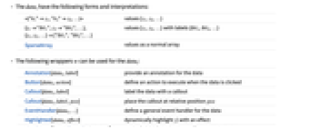
- datai 有以下形式和解释:
-
<|"k1"z1,"k2"z2,…|> 值 {z1,z2,…} {z1"lbl1",z2"lbl2",…}, {z1,z2,…}{"lbl1","lbl2",…} 带有标签 {lbl1,lbl2,…} 的值 {z1,z2,…} SparseArray 以数组形式给出的值 - ComplexListPlot[objcspec] 用列指定 cspec 从 Tabular、TimeSeries 或 EventSeries 对象 obj 中提取值并绘制.
- 可使用以下形式的列指定 cspec 来绘制表格数据:
-
col 绘制列 col 的 复数值 {col1,col2,…} 绘制列 col1、col2、… 的值 - 可对 datai 使用以下封装 w:
-
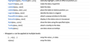
Annotation[datai,label] 为数据提供注释 Button[datai,action] 定义数据被点击时要执行的操作 Callout[datai,label] 用 callout 标记函数 Callout[datai,label,pos] 把 callout 放在相对位置 pos EventHandler[datai,…] 为数据定义通用事件处理器 Highlighted[datai,effect] 动态突出显示 fi 的效果 Highlighted[datai,Placed[effect,pos]] 静态突出显示 fi 在位置 pos 处的效果 Hyperlink[datai,uri] 将数据变为超链接 Labeled[datai,label] 标记数据 Labeled[datai,label,pos] 把标签放在相对位置 pos Legended[datai,label] 在图例中标识数据 PopupWindow[datai,cont] 为数据添加弹出窗口 StatusArea[datai,label] 当鼠标移过时在状态栏中显示 Style[datai,styles] 用指定样式显示数据 Tooltip[datai,label] 为数据添加提示条 Tooltip[datai] 将数据用作提示条 - 可在多个层级上应用封装 w:
-
{…,w[zi],…} 封装数据中的值 zi w[datai] 封装数据 w[{data1,…}] 封装一组 datai w1[w2[…]] 使用嵌套封装 - 在 Callout、Labeled 和 Placed 中可使用以下位置 pos:
-
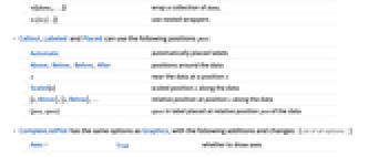
Automatic 自动放置标签 Above, Below, Before, After 数据周围的位置 x 在位置 x 处的数据周围 Scaled[s] 沿数据的缩放过的位置 s {s,Above},{s,Below},… 沿数据在位置 s 处的相对位置 {pos,epos} 在数据的相对位置 pos 处放置的标签中的 epos - ComplexListPlot 和 Graphics 有相同的选项,不同之处和更多选项如下所示: [所有选项的列表]
-
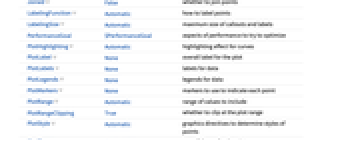
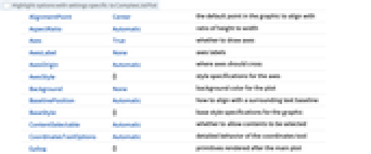
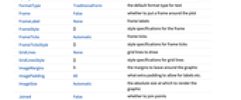
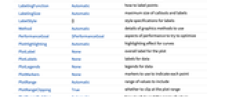
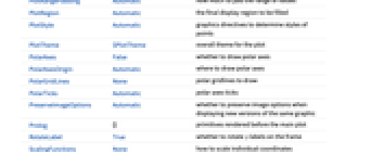
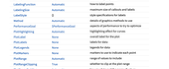
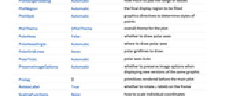
Axes True 是否绘制坐标轴 Joined False 是否将每个点都连起来 LabelingFunction Automatic 如何标记点 LabelingSize Automatic callout 和标签的最大尺寸 PerformanceGoal $PerformanceGoal 优化的目标 PlotHighlighting Automatic 突出显示曲线的效果 PlotLabel None 绘图的整体标签 PlotLabels None 数据的标签 PlotLegends None 数据的图例 PlotMarkers None 用于指明每个点的标记 PlotRange Automatic 包含的值范围 PlotRangeClipping True 在绘图范围边界处是否进行剪切 PlotStyle Automatic 确定点的样式的图形指令 PlotTheme $PlotTheme 绘图的整体外观主题 PolarAxes False 是否绘制极坐标轴 PolarAxesOrigin Automatic 在何处绘制极坐标轴 PolarGridLines None 极坐标网格线 PolarTicks Automatic 极坐标刻度 ScalingFunctions None 怎样缩放个别坐标 - LabelingFunction->f 指定了各点应有由 f[value,index,lbls] 给出的标签,其中 value 是与点相关的值、index 是它在 data 中的位置,而 lbls 是相关标签的列表.
- PlotLegends 的典型设置包括:
-
None 无图例 Automatic 自动确定图例 {lbl1,lbl2,…} 用 lbl1、lbl2、… 作为图例的标签 Placed[lspec,…] 指定图例的放置 - PlotStylesty 指定每条曲线使用的样式. 可能的设置包括:
-
{sty1,sty2,…} 针对各个数据集的一系列样式 <|"key"val,…|> 针对不同层级的数据的样式元素 - 接受的键有:
-
"Base" 所有 datai 的整体样式 "Lists" 针对每个 datai 的样式列表 styi - ColorData["DefaultPlotColors"] 给出 PlotStyle 使用的默认颜色序列.
- 为 MeshFunctions 中的函数提供的参数为 x、y、θ、r,其中 θ 和 r 是 zi 的辐角和半径. 默认情况下,为 ColorFunction 中的函数提供的是这些参数经过缩放的版本.
- Highlighted 和 PlotHighlighting 可能的突出显示效果包括:
-

style 突出显示指定的数据 

"Ball" 突出显示并标记数据中的指定点 

"Dropline" 突出显示并为数据中的指定点添加标签,并在轴线上标出垂线 

"XSlice" 突出显示并标记沿垂直切面的所有点 

"YSlice" 突出显示并标记沿水平切面的所有点 
Placed[effect,pos] 静态突出显示给定的位置 pos - 突出显示位置规格 pos 包括:
-
x, {x} {x,y} 处的效果,其中 y 为自动选择 {x,y} {x,y} 处的效果 {pos1,pos2,…} 多个位置 posi - ScalingFunctions->"scale" 缩放 zi 的模. ScalingFunctions{"scalex","scaley"} 分别缩放
和 imaginary 分量.
所有选项的列表
范例
打开所有单元 关闭所有单元基本范例 (4)

ComplexListPlot[{-2 - 2 I, -1 - I, 0, 1 + I, 2 + 2 I}]ComplexListPlot[{RandomComplex[{0, 1 + I}, 100], RandomComplex[{-2 - 2I, 2 + 2I}, 100]}]data = Table[a t Exp[2 π I t], {a, 2, 4}, {t, 0, 1, 0.02}];
ComplexListPlot[data, PlotLegends -> {"a=2", "a=3", "a=4"}]ComplexListPlot[Callout[#, #]& /@ Table[E^π I k / 4, {k, 1, 8}]]范围 (39)
数据 (7)
ComplexListPlot[Sin[Range[40] + 2I]]ComplexListPlot[{Sin[Range[40] + 2I], Cos[Range[40] + 2I]}]ComplexListPlot[{1 + I, 2 + 2I, Missing["NotAvailable"], 4 + 4I, None, 6 + 6I, ""}]用 MaxPlotPoints 限制所用点的个数:
data = Table[Exp[2Pi I RandomReal[]], {n, 200}];
Table[ComplexListPlot[data, MaxPlotPoints -> mp], {mp, {Infinity, 100, 50}}]自动选择 PlotRange:
{ComplexListPlot[{0, 1 + I, 2 + 2I, 3 + 3I, 4 + 20I, 5 + 5I, 20 + 6I}],
ComplexListPlot[{0, 1 + I, 2 + 2I, 3 + 3I, 4 + 20I, 5 + 5I, 20 + 6I}, PlotRange -> All]}用 PlotRange 显示感兴趣的区域:
{ComplexListPlot[{0, 1 + I, 2 + 2I, 3 + 3I, 4 + 100I, 5 + 5I, 20 + 6I}],
ComplexListPlot[{0, 1 + I, 2 + 2I, 3 + 3I, 4 + 100I, 5 + 5I, 20 + 6I}, PlotRange -> {0, 7 + 7I}]}用 ScalingFunctions 缩放坐标轴:
ComplexListPlot[Table[10^k + 2^kI, {k, -2, 5}], ScalingFunctions -> {"Log10", "Log2"}]表格数据 (1)
tab = Tabular[IconizedObject[«data»], {"seed", "solution", "basin"}]ComplexListPlot[tab -> "seed", PlotStyle -> AbsolutePointSize[2]]使用 PivotToColumns 为每个吸引盆(basin of attraction)生成列:
pivot = PivotToColumns[tab, "basin" -> "seed"]ComplexListPlot[pivot -> {Key[1], Key[2], Key[3]}, PlotStyle -> AbsolutePointSize[2]]特殊数据 (4)
ComplexListPlot[{1 + I -> "a", 2 + 2I -> "b", 3 + 3I -> "c", 4 + 4I -> "d", 5 + 3I -> "e", 6 + 2I -> "f", 7 + I -> "g"}]
ComplexListPlot[{1 + I, 2 + 2 I, 3 + 3 I, 4 + 4 I, 5 + 3 I, 6 + 2 I, 7 + I} -> {"a", "b", "c", "d", "e", "f", "g"}]ComplexListPlot[{1 + I, 2 + 2 I, 3 + 3 I, 4 + 4 I, 5 + 3 I, 6 + 2 I, 7 + I} -> {"a", "b", "c", "d", "e", "f", "g"}, LabelingFunction -> Above]将 Association 中的数值用作
坐标:
ComplexListPlot[<|"a" -> 2 + I, "b" -> 3 - I, "c" -> 5 + 2I, "d" -> 7, "e" -> 11 + 2I, "f" -> 13 - 3I|>]绘制 SparseArray 中的数据:
ComplexListPlot[SparseArray[RandomComplex[{0, 1 + I}, 25]]]封装 (6)
{ComplexListPlot[{{1 + I, Style[3 + 2I, Red], 6 + 3I}, {1 + 4I, 3 + 5I, 6 + 6I}}, PlotStyle -> PointSize[0.05]],
ComplexListPlot[{Style[{1 + I, 3 + 2I, 6 + 3I}, Red], {1 + 4I, 3 + 5I, 6 + 6I}}, PlotStyle -> PointSize[0.05]],
ComplexListPlot[Style[{{1 + I, 3 + 2I, 6 + 3I}, {1 + 4I, 3 + 5I, 6 + 6I}}, Red], PlotStyle -> PointSize[0.05]]}{ComplexListPlot[{{1 + I, Style[3 + 2I, Red], 6 + 3I}, {1 + 4I, 3 + 5I, 6 + 6I}}, PlotStyle -> PointSize[0.05]],
ComplexListPlot[{Style[{1 + I, Style[3 + 2I, Red], 6 + 3I}, Green], {1 + 4I, 3 + 5I, 6 + 6I}}, PlotStyle -> PointSize[0.05]],
ComplexListPlot[Style[{Style[{1 + I, Style[3 + 2I, Red], 6 + 3I}, Green], {1 + 4I, 3 + 5I, 6 + 6I}}, Blue], PlotStyle -> PointSize[0.05]]}ComplexListPlot[Tooltip[Table[k + Sqrt[k]I, {k, 10}], "square roots"]]ComplexListPlot[Table[Labeled[RandomComplex[{0, 1 + I}], i], {i, 20}], PlotStyle -> PointSize[Medium], ImageSize -> 300]用 PopupWindow 单击特征值以查看相应的特征向量:
{evalues, evecs} = Eigensystem[RandomComplex[{-1 - I, 1 + I}, {4, 4}]];
ComplexListPlot[PopupWindow@@@Transpose[{evalues, evecs}], PlotStyle -> PointSize[0.04]]可用 Button 触发操作:
evalues = Eigenvalues[RandomComplex[{-1 - I, 1 + I}, {8, 8}]];
ComplexListPlot[Button[#, Speak[#]]& /@ evalues, PlotStyle -> PointSize[0.02]]添加标签和图例 (15)
ComplexListPlot[Table[Labeled[RandomComplex[{0, 1 + I}], i], {i, 20}]]Table[ComplexListPlot[Table[Labeled[RandomComplex[{0, 1 + I}], i, p], {i, 20}], PlotLabel -> p], {p, {Above, Below, Before, After}}]用 Labeled 标记数据:
ComplexListPlot[{
Labeled[NestList[(0.9 + 0.1I)#&, 1 + I, 30], 0.1], Labeled[NestList[(0.9 + 0.2I)#&, 1 + I, 30], 0.2]
}]用 PlotLabels 标记数据:
ComplexListPlot[{
NestList[(0.9 + 0.1I)#&, 1 + I, 30], NestList[(0.9 + 0.2I)#&, 1 + I, 30]
}, PlotLabels -> {0.1, 0.2}]ComplexListPlot[{
Labeled[NestList[(0.9 + 0.1I)#&, 1 + I, 30], 0.1, 0.1], Labeled[NestList[(0.9 + 0.2I)#&, 1 + I, 30], 0.2, 0.3]
}]ComplexListPlot[{
Labeled[NestList[(0.9 + 0.1I)#&, 1 + I, 30], 0.1, Scaled[0.1]], Labeled[NestList[(0.9 + 0.2I)#&, 1 + I, 30], 0.2, Scaled[0.1]]
}]ComplexListPlot[{
Labeled[NestList[(0.9 + 0.1I)#&, 1 + I, 30], 0.1, {Scaled[0.1], Above}], Labeled[NestList[(0.9 + 0.2I)#&, 1 + I, 30], 0.2, {Scaled[0.1], Below}]
}]用 Callout 自动标记数据:
ComplexListPlot[{
Callout[NestList[(0.9 + 0.1I)#&, 1 + I, 30], 0.1], Callout[NestList[(0.9 + 0.2I)#&, 1 + I, 30], 0.2]
}]ComplexListPlot[{
Callout[NestList[(0.9 + 0.1I)#&, 1 + I, 30], 0.1, Above], Callout[NestList[(0.9 + 0.2I)#&, 1 + I, 30], 0.2, Below]
}]用 LabelingFunction 指定标签名:
ComplexListPlot[z /. Solve[z^6 == 1, z], LabelingFunction -> (DisplayForm[RowBox[{"(", #1[[1]], #1[[2]], ")"}]]&)]ComplexListPlot[z /. Solve[z^12 == 1, z], LabelingFunction -> (Arg[#1[[1]] + I#[[2]]]&)]Quiet@ComplexListPlot[z /. Solve[z^50 == 1, z], LabelingFunction -> (Arg[#1[[1]] + I#[[2]]]&)]Quiet@ComplexListPlot[z /. Solve[z^50 == 1, z], LabelingFunction -> (Arg[#1[[1]] + I#[[2]]]&), ImageSize -> 500]ComplexListPlot[{
NestList[(0.9 + 0.1I)#&, 1 + I, 30], NestList[(0.9 + 0.2I)#&, 1 + I, 30]
}, PlotLegends -> {0.1, 0.2}]用 Legended 为特定数据集提供图例:
matrix = RandomComplex[{-1 - I, 1 + I}, {10, 10}];
evals1 = Eigenvalues[matrix];
evals2 = Eigenvalues[(matrix + ConjugateTranspose[matrix]/2)];
ComplexListPlot[{evals1, Legended[evals2, "eigenvalues of the
symmetric matrix"]}]用 Placed 改变图例的位置:
ComplexListPlot[{evals1, Legended[evals2, Placed["eigenvalues of the symmetric matrix", Below]]}]ComplexListPlot[<|"random" -> evals1, "symmetric" -> evals2|>, PlotLabels -> Automatic]当你把鼠标移到绘图上方时,地图通常会有交互式 callouts 显示坐标:
ComplexListPlot[{IconizedObject[«data»], IconizedObject[«data2»]}]演示 (6)
f = (z^6 + z^3 + 1/z^10 - 1024);
zeros = z /. Solve[f == 0, z];
poles = z /. Solve[Denominator[f] == 0, z];
ComplexListPlot[{zeros, poles}]ComplexListPlot[{zeros, poles}, PlotStyle -> {Blue, Red}]ComplexListPlot[{zeros, poles}, PlotTheme -> "Marketing"]ComplexListPlot[{zeros, poles}, PlotLegends -> {"zeros", "poles"}]用 Legended 为特定数据集提供图例:
ComplexListPlot[{zeros, Legended[poles, "poles"]}]为数据提供交互 Tooltip:
ComplexListPlot[Table[Tooltip[Exp[2Pi I k / 10], Exp[2Pi I k / 10]], {k, 0, 9}]]ComplexListPlot[Table[Exp[2Pi I k / n], {n, {3, 5, 7}}, {k, 0, n - 1}], PlotMarkers -> Automatic]ComplexListPlot[Table[Exp[2Pi I k / n], {n, {3, 5, 7}}, {k, 0, n - 1}], PlotMarkers -> {"3", "5", "7"}]通过 Joined 将各点连成线:
ComplexListPlot[Table[Exp[2Pi I k / 10], {k, 0, 10}], Joined -> True]用 InterpolationOrder 使数据更平滑:
Table[ComplexListPlot[Table[Exp[2Pi I k / 10], {k, 0, 10}], Joined -> True, InterpolationOrder -> io], {io, {0, 1, 2}}]选项 (156)
AspectRatio (4)
ComplexListPlot[Table[x + I Sin[x], {x, 0, 2Pi, 0.1}]]ComplexListPlot[Table[x + I Sin[x], {x, 0, 2Pi, 0.1}], AspectRatio -> 1 / GoldenRatio]设置 AspectRatio1 可使高度与宽度相同:
ComplexListPlot[Table[x + I Sin[x], {x, 0, 2Pi, 0.1}], AspectRatio -> 1]AspectRatioFull 调整高度和宽度以紧密贴合其他构造:
plot = ComplexListPlot[Table[x + I Sin[x], {x, 0, 2Pi, 0.1}], AspectRatio -> Full];
{Framed[Pane[plot, {75, 100}]], Framed[Pane[plot, {100, 100}]], Framed[Pane[plot, {100, 50}]]}Axes (3)
默认情况下,ComplexListPlot 绘制轴:
ComplexListPlot[Table[x + I Sin[x], {x, 0, 2 π, 0.1}]]使用 AxesOrigin 可指定轴相交处:
ComplexListPlot[Table[x + I Sin[x], {x, 0, 2 π, 0.1}], Frame -> False, Axes -> True, AxesOrigin -> {0, 0}]{ComplexListPlot[Table[x + I Sin[x], {x, 0, 2 π, 0.1}], Axes -> {True, False}], ComplexListPlot[Table[x + I Sin[x], {x, 0, 2 π, 0.1}], Axes -> {False, True}]}AxesLabel (3)
AxesOrigin (2)
AxesStyle (4)
ComplexListPlot[Table[x + I Sin[x], {x, 0, 2 π, 0.1}], Frame -> False, Axes -> True, AxesStyle -> Red]ComplexListPlot[Table[x + I Sin[x], {x, 0, 2 π, 0.1}], Frame -> False, Axes -> True, AxesStyle -> {{Thick, Red}, {Thick, Blue}}]ComplexListPlot[Table[x + I Sin[x], {x, 0, 2 π, 0.1}], Frame -> False, Axes -> True, AxesStyle -> Green, TicksStyle -> StandardGray]ComplexListPlot[Table[x + I Sin[x], {x, 0, 2 π, 0.1}], Frame -> False, Axes -> True, AxesStyle -> Green, LabelStyle -> StandardGray]ClippingStyle (4)
ClippingStyle 要求至少要有一个数据集是 Joined:
{ComplexListPlot[Table[x + I Sin[x] / x ^ 2, {x, -10, 10, 0.2}], ClippingStyle -> Red],
ComplexListPlot[Table[x + I Sin[x] / x ^ 2, {x, -10, 10, 0.2}], ClippingStyle -> Red, Joined -> True]}//QuietComplexListPlot[Table[x + I Sin[x] / x ^ 2, {x, -10, 10, 0.2}], ClippingStyle -> None, Joined -> True]//Quiet在底部用红线显示被剪掉的区域,在顶部用粗线显示被剪掉的区域:
ComplexListPlot[Table[x + I Sin[x] / x ^ 2, {x, -10, 10, 0.2}], ClippingStyle -> {Red, Thick}, Joined -> True]//QuietComplexListPlot[Table[x + I Sin[x] / x ^ 2, {x, -10, 10, 0.2}], ClippingStyle -> Directive[Red, Thick], Joined -> True]//QuietColorFunction (3)
Table[ComplexListPlot[Table[Sin[2x]Exp[I x], {x, 0, 2π, .1}], Joined -> True, PlotLabel -> Hue[var], ColorFunction -> Function[{x, y, θ, r}, Evaluate[Hue[var]]]], {var, {x, y, θ, r}}]对于曲线着色,ColorFunction 比 PlotStyle 的优先级高:
ComplexListPlot[Table[t Exp[I t], {t, 0, 4Pi, .1}], ColorFunction -> "Rainbow", Joined -> True, PlotStyle -> Directive[Red, Thick]]在 MeshShading 中设置 Automatic 以使用 ColorFunction:
ComplexListPlot[Table[t Exp[I t], {t, 0, 4Pi, .1}], ColorFunction -> "Rainbow", Joined -> True, PlotStyle -> Directive[Red, Thick], Mesh -> 10, MeshShading -> {Automatic, StandardGray}, MeshStyle -> None]ColorFunctionScaling (4)
ColorFunctionScaling 要求至少要有一个数据集是 Joined:
{ComplexListPlot[Table[t Exp[I t], {t, 0, 4Pi, .1}], ColorFunction -> "Rainbow", ColorFunctionScaling -> True],
ComplexListPlot[Table[t Exp[I t], {t, 0, 4Pi, .1}], ColorFunction -> "Rainbow", ColorFunctionScaling -> True, Joined -> True]}ComplexListPlot[Table[0.25(I + Exp[I t]), {t, 0, 2Pi, .1}], ColorFunction -> Function[{x, y}, Hue[y]], Joined -> True, ColorFunctionScaling -> True]ComplexListPlot[Table[0.25(I + Exp[I t]), {t, 0, 2Pi, .1}], ColorFunction -> Function[{x, y}, Hue[y]], Joined -> True, ColorFunctionScaling -> False]Table[ComplexListPlot[Table[Sin[2x]Exp[I x], {x, 0, 2π, .05}], Joined -> True, ColorFunctionScaling -> False, PlotLabel -> Hue[var], ColorFunction -> Function[{x, y, θ, r}, Evaluate[Hue[var]]]], {var, {x, y, θ, r}}]Frame (3)
ComplexListPlot[Table[x + I Sin[x], {x, 0, 2 Pi, 0.1}], AspectRatio -> 1, Frame -> True]ComplexListPlot[Table[x + I Sin[x], {x, 0, 2 Pi, 0.1}], AspectRatio -> 1, Frame -> {{True, True}, {False, False}}]ComplexListPlot[Table[x + I Sin[x], {x, 0, 2 Pi, 0.1}], AspectRatio -> 1, Frame -> {{True, False}, {True, False}}]FrameLabel (4)
ComplexListPlot[Table[x + I Sin[x], {x, 0, 2 Pi, 0.1}], AspectRatio -> 1, Frame -> True, FrameLabel -> {"label"}]ComplexListPlot[Table[x + I Sin[x], {x, 0, 2 Pi, 0.1}], AspectRatio -> 1, Frame -> True, FrameLabel -> {"bottom", "left"}]ComplexListPlot[Table[x + I Sin[x], {x, 0, 2 Pi, 0.1}], AspectRatio -> 1, Frame -> True, FrameLabel -> {{"left", "right"}, {"bottom", "top"}}]ComplexListPlot[Table[x + I Sin[x], {x, 0, 2 Pi, 0.1}], AspectRatio -> 1, Frame -> True, FrameLabel -> {{"left", "right"}, {"bottom", "top"}}, LabelStyle -> Directive[Bold, Red]]FrameStyle (2)
ComplexListPlot[Table[x + I Sin[x], {x, 0, 2 Pi, 0.1}], AspectRatio -> 1, Frame -> True, FrameStyle -> Directive[StandardGray, Thick]]ComplexListPlot[Table[x + I Sin[x], {x, 0, 2 Pi, 0.1}], AspectRatio -> 1, Frame -> True, FrameStyle -> {{Directive[Green, Thick], Directive[Red]}, {Directive[Gray, Thick], Directive[Blue]}}]FrameTicks (9)
ComplexListPlot[Table[x + I Sin[x], {x, 0, 2 Pi, 0.1}], AspectRatio -> 1, Frame -> True]ComplexListPlot[Table[x + I Sin[x], {x, 0, 2 Pi, 0.1}], AspectRatio -> 1, Frame -> True, FrameTicks -> None]ComplexListPlot[Table[x + I Sin[x], {x, 0, 2 Pi, 0.1}], AspectRatio -> 1, Frame -> True, FrameTicks -> {{None, None}, {Automatic, None}}]ComplexListPlot[Table[x + I Sin[x], {x, 0, 2 Pi, 0.1}], AspectRatio -> 1, Frame -> True, FrameTicks -> Automatic]使用 All 可在所有边上添加刻度标签:
ComplexListPlot[Table[x + I Sin[x], {x, 0, 2 Pi, 0.1}], AspectRatio -> 1, Frame -> True, FrameTicks -> All]ComplexListPlot[Table[x + I Sin[x], {x, 0, 2 Pi, 0.1}], AspectRatio -> 1, Frame -> True, FrameTicks -> {{{1, .5, -1}, Automatic}, {{1, Pi, 4}, Automatic}}]ComplexListPlot[Table[x + I Sin[x], {x, 0, 2 Pi, 0.1}], AspectRatio -> 1, Frame -> True, FrameTicks -> {{{{1, a}, {.5, b}, {-1, -a}}, Automatic}, {{{1, a}, {Pi, "Pi"}, {6, d}}, Automatic}}]ComplexListPlot[Table[x + I Sin[x], {x, 0, 2 Pi, 0.1}], AspectRatio -> 1, Frame -> True, FrameTicks -> {{{{1, a}, {.5, b}, {-1, -a}}, Automatic}, {{{1, a, 0.86}, {Pi, "Pi", 0.5}, {6, d, .4}}, Automatic}}]ComplexListPlot[Table[x + I Sin[x], {x, 0, 2 Pi, 0.1}], AspectRatio -> 1, Frame -> True, FrameTicks -> {{{{1, a}, {.5, b}, {-1, -a}}, Automatic}, {{{1, a, {0.86, 0.05}}, {Pi, Pi, {0.5, 0.1}}, {6, d, {.4, .2}}}, Automatic}}]ComplexListPlot[Table[x + I Sin[x], {x, 0, 2 Pi, 0.1}], AspectRatio -> 1, Frame -> True, FrameTicks -> {{{{1, a}, {.5, b}, {-1, -a}}, Automatic}, {{{1, a, 0.86, Directive[Red, Thick]}, {Pi, "Pi", 0.5, Directive[StandardGray, Thick, Dashed]}, {6, d, .4, Darker@Green}}, Automatic}}]minMeanMax[min_, max_] := {{min, min}, {(max + min) / 2, (max + min) / 2}, {max, max}}ComplexListPlot[Table[x + I Sin[x], {x, 0, 2 Pi, 0.1}], AspectRatio -> 1, Frame -> True, FrameTicks -> {{minMeanMax, None}, {minMeanMax, None}}, PlotRangePadding -> None]FrameTicksStyle (3)
ComplexListPlot[Table[x + I Sin[x], {x, 0, 2 Pi, 0.1}], AspectRatio -> 1, Frame -> True, FrameStyle -> Directive[Red]]ComplexListPlot[Table[x + I Sin[x], {x, 0, 2 Pi, 0.1}], AspectRatio -> 1, Frame -> True, FrameStyle -> Directive[Red], FrameTicksStyle -> Directive[Blue, Thick]]ComplexListPlot[Table[x + I Sin[x], {x, 0, 2 Pi, 0.1}], AspectRatio -> 1, Frame -> True, FrameTicks -> All, FrameTicksStyle -> {{Purple, Blue}, {Thick, Red}}]ImageSize (8)
使用有名称的尺寸如 Tiny、Small、Medium 和 Large:
{ComplexListPlot[Table[x + I Sin[x], {x, 0, 2Pi, 0.1}], ImageSize -> Tiny], ComplexListPlot[Table[x + I Sin[x], {x, 0, 2Pi, 0.1}], ImageSize -> Small]}{ComplexListPlot[Table[x + I Sin[x], {x, 0, 2Pi, 0.1}], ImageSize -> 150], ComplexListPlot[Table[x + I Sin[x], {x, 0, 2Pi, 0.1}], AspectRatio -> 1.5, ImageSize -> 150]}{ComplexListPlot[Table[x + I Sin[x], {x, 0, 2Pi, 0.1}], ImageSize -> {Automatic, 150}], ComplexListPlot[Table[x + I Sin[x], {x, 0, 2Pi, 0.1}], AspectRatio -> 1.5, ImageSize -> {Automatic, 150}]}{ComplexListPlot[Table[x + I Sin[x], {x, 0, 2Pi, 0.1}], ImageSize -> UpTo[200]], ComplexListPlot[Table[x + I Sin[x], {x, 0, 2Pi, 0.1}], AspectRatio -> 2, ImageSize -> UpTo[200]]}ComplexListPlot[Table[x + I Sin[x], {x, 0, 2Pi, 0.1}], ImageSize -> {200, 200}, Background -> StandardBlue]设置 AspectRatioFull 会填充可用空间:
ComplexListPlot[Table[x + I Sin[x], {x, 0, 2Pi, 0.1}], AspectRatio -> Full, ImageSize -> {200, 200}, Background -> StandardBlue]{ComplexListPlot[Table[x + I Sin[x], {x, 0, 2Pi, 0.1}], ImageSize -> {UpTo[150], UpTo[100]}], ComplexListPlot[Table[x + I Sin[x], {x, 0, 2Pi, 0.1}], AspectRatio -> 2, ImageSize -> {UpTo[150], UpTo[100]}]}设置 ImageSizeFull 会填充对象中的可用空间:
Framed[Pane[ComplexListPlot[Table[x + I Sin[x], {x, 0, 2Pi, 0.1}], ImageSize -> Full, Background -> StandardBlue], {200, 100}]]Framed[Pane[ComplexListPlot[Table[x + I Sin[x], {x, 0, 2Pi, 0.1}], ImageSize -> {Scaled[0.5], Scaled[0.5]}, Background -> StandardBlue], {200, 100}]]data = RandomComplex[{0, 10 + 10I}, 200] -> Range[200];ComplexListPlot[data]ComplexListPlot[data, ImageSize -> 200]ComplexListPlot[data, ImageSize -> 500]InterpolationOrder (4)
InterpolationOrder 要求至少要有一个数据集是 Joined:
{ComplexListPlot[Table[t Exp[I t], {t, 0, 4Pi, 1}], InterpolationOrder -> 2], ComplexListPlot[Table[t Exp[I t], {t, 0, 4Pi, 1}], InterpolationOrder -> 2, Joined -> True]}ComplexListPlot[Table[t Exp[I t], {t, 0, 4Pi, 1}], Joined -> True, InterpolationOrder -> None, Mesh -> Full]ComplexListPlot[Table[t Exp[I t], {t, 0, 4Pi, 1}], Joined -> True, InterpolationOrder -> 0, Mesh -> Full]Table[ComplexListPlot[Table[t Exp[I t], {t, 0, 4Pi, 1}], Joined -> True, InterpolationOrder -> i, Mesh -> Full, PlotLabel -> i], {i, 0, 3}]Joined (3)
data = Table[t Exp[2π I t], {t, 0, 10, .1}];
Table[ComplexListPlot[data, Joined -> s], {s, {False, True}}]用线连接第一个数据集中的点,但用点显示第二个数据集中的数据:
ComplexListPlot[Table[40BesselJ[n, x] + I BesselI[n, x], {n, 1, 2}, {x, 0, 5, .1}], Joined -> {True, False}]ComplexListPlot[Table[40BesselJ[1, x] + I BesselI[1, x], {x, 0, 5, .1}], Joined -> True, Mesh -> All]LabelingFunction (7)
如果值和标签的列表长度相同,则可用 Rule 对点进行标注:
ComplexListPlot[{1, E^(2 I π/7), E^(4 I π/7), E^(6 I π/7), E^(8 I π/7), E^(10 I π/7), E^(12 I π/7)} -> {0, 1, 2, 3, 4, 5, 6}]ComplexListPlot[{1 -> 0, E^(2 I π/7) -> 1, E^(4 I π/7) -> 2, E^(6 I π/7) -> 3, E^(8 I π/7), E^(10 I π/7), E^(12 I π/7)}]用 LabelingFunctionNone 即可不显示标签:
ComplexListPlot[{1, E^(2 I π/7), E^(4 I π/7), E^(6 I π/7), E^(8 I π/7), E^(10 I π/7), E^(12 I π/7)} -> {0, 1, 2, 3, 4, 5, 6}, LabelingFunction -> None]ComplexListPlot[{1, E^(2 I π/7), E^(4 I π/7), E^(6 I π/7), E^(8 I π/7), E^(10 I π/7), E^(12 I π/7)} -> {0, 1, 2, 3, 4, 5, 6}, LabelingFunction -> Above]放置在 Tooltip 中:
ComplexListPlot[{1, E^(2 I π/7), E^(4 I π/7), E^(6 I π/7), E^(8 I π/7), E^(10 I π/7), E^(12 I π/7)} -> {0, 1, 2, 3, 4, 5, 6}, LabelingFunction -> Tooltip]ComplexListPlot[{1, E^(2 I π/7), E^(4 I π/7), E^(6 I π/7), E^(8 I π/7), E^(10 I π/7), E^(12 I π/7)}, LabelingFunction -> (DisplayForm[ToBoxes[TraditionalForm[#1]] /. {"{" -> "(", "}" -> ")"}]&)]ComplexListPlot[{1, E^(2 I π/7), E^(4 I π/7), E^(6 I π/7), E^(8 I π/7), E^(10 I π/7), E^(12 I π/7)}, LabelingFunction -> (Last[#2] - 1&)]LabelingSize (3)
ComplexListPlot[{1, E^(2 I π/7), E^(4 I π/7), E^(6 I π/7), E^(8 I π/7), E^(10 I π/7), E^(12 I π/7)} -> {"zeroth", "first", "second", "third", "fourth", "fifth", "sixth"}]ComplexListPlot[{1, E^(2 I π/7), E^(4 I π/7), E^(6 I π/7), E^(8 I π/7), E^(10 I π/7), E^(12 I π/7)} -> {"zeroth", "first", "second", "third", "fourth", "fifth", "sixth"}, LabelingSize -> 25]images = {[image], [image], [image], [image], [image], [image], [image]};ComplexListPlot[{1, E^(2 I π/7), E^(4 I π/7), E^(6 I π/7), E^(8 I π/7), E^(10 I π/7), E^(12 I π/7)} -> images]ComplexListPlot[{1, E^(2 I π/7), E^(4 I π/7), E^(6 I π/7), E^(8 I π/7), E^(10 I π/7), E^(12 I π/7)} -> images, LabelingSize -> 50]ComplexListPlot[{1, E^(2 I π/7), E^(4 I π/7), E^(6 I π/7), E^(8 I π/7), E^(10 I π/7), E^(12 I π/7)} -> images, ImageSize -> 72 8, LabelingSize -> Full]MaxPlotPoints (1)
用 MaxPlotPoints 限制所用的点的数量:
data = Table[k Exp[2Pi I k / 100], {k, 200}];
Table[ComplexListPlot[data, MaxPlotPoints -> mp], {mp, {Infinity, 100, 50}}]Mesh (6)
{ComplexListPlot[Table[t Exp[I t], {t, 20}], Mesh -> 10], ComplexListPlot[Table[t Exp[I t], {t, 20}], Mesh -> 10, Joined -> True]}{ComplexListPlot[Table[t Exp[I t], {t, 20}], Mesh -> Full, Joined -> True], ComplexListPlot[Table[t Exp[I t], {t, 20}], Mesh -> All, Joined -> True]}{ComplexListPlot[Table[t Exp[I t], {t, 20}], Mesh -> Full, Joined -> True, InterpolationOrder -> 2], ComplexListPlot[Table[t Exp[I t], {t, 20}], Mesh -> All, Joined -> True, InterpolationOrder -> 2]}ComplexListPlot[Table[t Exp[I t], {t, 20}], Mesh -> 20, Joined -> True]ComplexListPlot[Table[t Exp[I t], {t, 20}], Mesh -> {{-9, 1, 2, 5, 8}}, Joined -> True]ComplexListPlot[Table[t Exp[I t], {t, 20}], Mesh -> {Table[{x, Directive[Hue[x / 20], PointSize[Large]]}, {x, -10, 10}]}, Joined -> True, ColorFunction -> (Hue[#1 / 20]&), ColorFunctionScaling -> False]MeshFunctions (3)
MeshFunctions 要求至少要有一个数据集是 Joined:
{ComplexListPlot[Table[t Exp[I t], {t, 20}], Mesh -> 10, MeshFunctions -> {#1&}], ComplexListPlot[Table[t Exp[I t], {t, 20}], Mesh -> 10, MeshFunctions -> {#1&}, Joined -> True]}在
方向上显示 5 个网格(红色),在
方向上显示 10 个网格(蓝色):
ComplexListPlot[Table[t Exp[I t], {t, 20}], Joined -> True, Mesh -> {5, 10}, MeshFunctions -> {#1&, #2&}, MeshStyle -> {Directive[PointSize[Large], Red], Directive[PointSize[Medium], Blue]}]Table[ComplexListPlot[Table[Sin[2 x] Exp[I x], {x, 0, 2 π, .05}], Joined -> True, Mesh -> 5, MeshStyle -> AbsolutePointSize[5], MeshFunctions -> Function[{x, y, θ, r}, Evaluate[var]], PlotLabel -> var], {var, {x, y, θ, r}}]MeshShading (7)
MeshShading 要求至少要有一个数据集是 Joined:
{ComplexListPlot[Table[t Exp[I t], {t, 20}], Mesh -> 10, MeshShading -> {Red, Blue}], ComplexListPlot[Table[t Exp[I t], {t, 20}], Mesh -> 10, MeshShading -> {Red, Blue}, Joined -> True]}ComplexListPlot[Table[t Exp[I t], {t, 20}], Mesh -> 10, MeshFunctions -> {#1&}, MeshShading -> {Red, Blue}, Joined -> True]用 None 移除线段:
ComplexListPlot[Table[t Exp[I t], {t, 20}], Mesh -> 10, MeshFunctions -> {#1&}, MeshShading -> {Red, None}, Joined -> True]MeshShading 可与 PlotStyle 一起使用:
ComplexListPlot[Table[t Exp[I t], {t, 20}], Mesh -> 10, MeshFunctions -> {#1&}, MeshShading -> {Red, Blue}, PlotStyle -> Dashed, Joined -> True]MeshShading 比 PlotStyle 的优先级高:
ComplexListPlot[Table[t Exp[I t], {t, 20}], Mesh -> 10, MeshFunctions -> {#1&}, MeshShading -> {Red, Blue}, PlotStyle -> Green, Joined -> True]通过将 MeshShading 设为 Automatic 对某些线段使用 PlotStyle:
ComplexListPlot[Table[t Exp[I t], {t, 20}], Mesh -> 10, MeshFunctions -> {#1&}, MeshShading -> {Red, Automatic}, PlotStyle -> StandardBlue, Joined -> True]MeshShading 可与 ColorFunction一起使用:
ComplexListPlot[Table[t Exp[I t], {t, 20}], Mesh -> 10, MeshFunctions -> {#1&}, MeshShading -> {StandardGray, Automatic}, ColorFunction -> Function[{x, y}, Hue[x]], Joined -> True]PlotHighlighting (7)
在默认设置 PlotHighlightingAutomatic 下,绘图有交互式坐标 callout:
ComplexListPlot[Table[40BesselJ[2, x] + I BesselI[2, x], {x, 0, 5, .1}]]设置 PlotHighlightingNone 可禁用整个绘图的突出显示:
ComplexListPlot[Table[40BesselJ[2, x] + I BesselI[2, x], {x, 0, 5, .1}], PlotHighlighting -> None]使用 Highlighted[…,None] 可仅禁用单个数据组的突出显示:
ComplexListPlot[{Table[40BesselJ[2, x] + I BesselI[2, x], {x, 0, 5, .2}], Highlighted[Table[40BesselJ[3, x] + I BesselI[3, x], {x, 0, 5, .2}], None]}]ComplexListPlot[{Table[40BesselJ[2, x] + I BesselI[2, x], {x, 0, 5, .2}], Table[40BesselJ[3, x] + I BesselI[3, x], {x, 0, 5, .2}]}, PlotHighlighting -> Directive[Red, AbsolutePointSize[10], DropShadowing[]]]ComplexListPlot[Table[40BesselJ[2, x] + I BesselI[2, x], {x, 0, 5, .2}], PlotHighlighting -> "Dropline"]ComplexListPlot[Table[40BesselJ[2, x] + I BesselI[2, x], {x, 0, 5, .2}], PlotHighlighting -> "Dropline"]ComplexListPlot[Table[40BesselJ[2, x] + I BesselI[2, x], {x, 0, 5, .1}], PlotHighlighting -> "XNearestPoint"]ComplexListPlot[Table[40BesselJ[2, x] + I BesselI[2, x], {x, 0, 5, .1}], PlotHighlighting -> {"XNearestPoint", <|"Style" -> Green|>}]ComplexListPlot[Table[40BesselJ[2, x] + I BesselI[2, x], {x, 0, 5, .1}], PlotHighlighting -> "XYLabel"]使用 Callout 选项改变标签外观:
ComplexListPlot[Table[40BesselJ[2, x] + I BesselI[2, x], {x, 0, 5, .1}], PlotHighlighting -> {"XYLabel", <|"Appearance" -> "Corners", "CalloutMarker" -> "Circle"|>}]ComplexListPlot[Table[40BesselJ[2, x] + I BesselI[2, x], {x, 0, 5, .1}], PlotHighlighting -> {{"XNearestPoint", <|"Style" -> StandardGray|>}, {"XYLabel", <|"Appearance" -> "Corners", "CalloutMarker" -> "Circle"|>}}]PlotLabel (1)
PlotLabels (5)
ComplexListPlot[{Sin[Range[20] + 2I], Range[-5, 10] + 2I}, PlotLabels -> {"circle", "line"}]ComplexListPlot[{Sin[Range[20] + 2I], Range[-5, 10] + 2I}, PlotLabels -> Placed[{"circle", "line"}, Above]]ComplexListPlot[{Sin[Range[20] + 2I], Range[-5, 10] + 2I}, PlotLabels -> {Callout["circle", {Scaled[0.25], Above}], Callout["line", {Scaled[0.25], Below}]}]用 Association 的键作为标签:
ComplexListPlot[<|"circle" -> Sin[Range[20] + 2I], "line" -> Range[-5, 10] + 2I|>, PlotLabels -> Automatic, PlotLegends -> False]用 None 不添加标签:
ComplexListPlot[{Sin[Range[20] + 2I], Range[-5, 10] + 2I}, PlotLabels -> {None, "line"}]PlotLegends (6)
ComplexListPlot[{Sin[Range[20] + 2I], Range[-5, 10] + 2I}, PlotLegends -> {"circle", "line"}]ComplexListPlot[{Sin[Range[20] + 2I], Range[-5, 10] + 2I}, PlotLegends -> Automatic]ComplexListPlot[{Sin[Range[20] + 2I], Range[-5, 10] + 2I}, PlotLegends -> {"circle", "line"}, PlotStyle -> {Red, Blue}]用 Placed 指定图例的放置:
Table[ComplexListPlot[{Sin[Range[20] + 2I], Range[-5, 10] + 2I}, PlotLegends -> Placed[{"circle", "line"}, pos], PlotStyle -> {Red, Blue}], {pos, {Above, Below, Before, After}}]ComplexListPlot[{Sin[Range[20] + 2I], Range[-5, 10] + 2I}, PlotLegends -> Placed[{"circle", "line"}, {0.85, 0.25}], PlotStyle -> {Red, Blue}]用 PlotLegends 改变外观:
ComplexListPlot[{Sin[Range[20] + 2I], Range[-5, 10] + 2I}, PlotLegends -> PointLegend[{"circle", "line"}, LegendMarkerSize -> 10, LegendFunction -> Frame]]PlotMarkers (8)
ComplexListPlot 通常用不同的颜色来区分不同的数据集:
ComplexListPlot[Table[Sin[2(t + p)]Exp[I (t + p)], {p, 0, 3Pi / 2, Pi / 2}, {t, 0, Pi / 2, 0.05}], PlotMarkers -> None]ComplexListPlot[Table[Sin[2(t + p)]Exp[I (t + p)], {p, 0, 3Pi / 2, Pi / 2}, {t, 0, Pi / 2, 0.05}], PlotMarkers -> Automatic]ComplexListPlot[Table[Sin[2(t + p)]Exp[I (t + p)], {p, 0, 3Pi / 2, Pi / 2}, {t, 0, Pi / 2, 0.05}], PlotMarkers -> Automatic, PlotStyle -> StandardBlue]Table[ComplexListPlot[Table[Sin[2(t + p)]Exp[I (t + p)], {p, 0, 3Pi / 2, Pi / 2}, {t, 0, Pi / 2, 0.05}], PlotMarkers -> {Automatic, s}], {s, {Small, Medium, Large}}]ComplexListPlot[Table[Sin[2(t + p)]Exp[I (t + p)], {p, 0, 3Pi / 2, Pi / 2}, {t, 0, Pi / 2, 0.05}], PlotMarkers -> {"1", "2", "3", "4"}]{m1, m2, m3, m4} = Graphics /@ {Circle[{0, 0}, 1], Disk[{0, 0}, 1], Line[{{-0.5, -0.5}, {0.5, -0.5}, {0.5, 0.5}, {-0.5, 0.5}, {-0.5, -0.5}}], Polygon[{{-0.5, -0.5}, {0.5, -0.5}, {0, Sqrt[3] / 4}}]}ComplexListPlot[Table[Sin[2(t + p)]Exp[I (t + p)], {p, 0, 3Pi / 2, Pi / 2}, {t, 0, Pi / 2, 0.05}], PlotMarkers -> Table[{s, 0.03}, {s, {m1, m2, m3, m4}}]]ComplexListPlot[Table[Sin[2(t + p)]Exp[I (t + p)], {p, 0, 3Pi / 2, Pi / 2}, {t, 0, Pi / 2, 0.05}], PlotMarkers -> "●"]Table[ComplexListPlot[Table[Sin[2(t + p)]Exp[I (t + p)], {p, 0, 3Pi / 2, Pi / 2}, {t, 0, Pi / 2, 0.05}], PlotMarkers -> {"●", s}], {s, {4, 8, 12}}]PlotRange (4)
自动计算 PlotRange:
ComplexListPlot[Fourier[Table[Cos[2 π 3 t], {t, 0, 2, 0.05}]]]ComplexListPlot[Fourier[Table[Cos[2 π 3 t], {t, 0, 2, 0.05}]], PlotRange -> All]ComplexListPlot[Fourier[Table[Cos[2 π 3 t], {t, 0, 2, 0.05}]], PlotRange -> {{-3, 3}, {-2, 2}}]ComplexListPlot[Fourier[Table[Cos[2 π 3 t], {t, 0, 2, 0.05}]], PlotRange -> {-3 - 2I, 3 + 2I}]PlotStyle (7)
Table[ComplexListPlot[Table[Sin[3x]Exp[I x], {x, 0, Pi, 0.05}], PlotStyle -> ps], {ps, {Red, PointSize[Large], Darker[Green], Directive[Red, PointSize[Large]]}}]ComplexListPlot[Table[c Sin[3 x]Exp[I x], {c, 3}, {x, 0, Pi, 0.05}]]ComplexListPlot[Table[c Sin[3 x]Exp[I x], {c, 3}, {x, 0, Pi, 0.05}], PlotStyle -> {Red, Green, Blue}]将 PlotStyle 应用于曲线和点:
ComplexListPlot[Table[c Sin[3 x]Exp[I x], {c, 3}, {x, 0, Pi, 0.05}], PlotStyle -> {Red, Green, Blue}, Joined -> {False, True, False}]PlotStyle 可与 ColorFunction 一起使用:
ComplexListPlot[Table[c Sin[3 x]Exp[I x], {c, 3}, {x, 0, Pi, 0.05}], PlotStyle -> Thick, Joined -> True, ColorFunction -> Function[{x, y}, Hue[x]]]PlotStyle 可与 MeshShading 一起使用:
ComplexListPlot[Table[c Sin[3 x]Exp[I x], {c, 3}, {x, 0, Pi, 0.05}], PlotStyle -> Dashed, Joined -> True, Mesh -> 10, MeshFunctions -> {#3&}, MeshShading -> {Red, Blue}]默认情况下,MeshStyle 采用和 PlotStyle 相同的样式:
ComplexListPlot[Table[c Sin[3 x]Exp[I x], {c, 3}, {x, 0, Pi, 0.05}], PlotStyle -> Red, Joined -> True, Mesh -> All]PlotTheme (2)
PolarAxes (2)
PolarAxesOrigin (2)
ComplexListPlot[Table[(1 + 3Sin[4t])Exp[I t], {t, 0, 6π, .05}], PolarAxes -> True, PolarGridLines -> True, PolarAxesOrigin -> {0, 6}]ComplexListPlot[Table[(1 + 3Sin[4t])Exp[I t], {t, 0, 6π, .05}], PolarAxes -> True, PolarGridLines -> True, PolarAxesOrigin -> {{Right, Up}, Automatic}, PolarTicks -> {None, Automatic}]PolarGridLines (2)
ComplexListPlot[Table[Sin[4t]Exp[I t], {t, 0, 6π, .05}], PolarAxes -> True, PolarGridLines -> True]ComplexListPlot[Table[2Sin[4t]Exp[I t], {t, 0, 6π, .05}], PolarAxes -> {True, False}, PolarGridLines -> {Range[0, 2Pi, Pi / 4], {1, 2}}, PolarTicks -> {"Degrees", None}]ComplexListPlot[Table[2Sin[4t]Exp[I t], {t, 0, 6π, .05}], PolarAxes -> {False, True}, PolarGridLines -> {Range[0, 2Pi, Pi / 4], {1, 2}}, PolarTicks -> {None, Automatic}, GridLinesStyle -> Orange]PolarTicks (4)
ComplexListPlot[Table[5Cos[2t]Exp[I t], {t, 0, 6π, .05}], PolarAxes -> Automatic, PolarTicks -> Automatic]ComplexListPlot[Table[5Cos[2t]Exp[I t], {t, 0, 6π, .05}], PolarAxes -> Automatic, PolarTicks -> {Range[-Pi + Pi / 12, Pi, Pi / 12], Automatic}]ComplexListPlot[Table[5Cos[2t]Exp[I t], {t, 0, 6π, .05}], PolarAxes -> Automatic, PolarTicks -> {"Degrees", Automatic}]ComplexListPlot[Table[6Cos[2t]Exp[I t], {t, 0, 6π, .05}], PolarAxes -> {True, True}, PolarTicks -> {Range[0, 2Pi - Pi / 4, Pi / 4], Range[0, 10, 2]}]ScalingFunctions (3)
ComplexListPlot[Table[(10I)^t, {t, -5, 6}], Joined -> True, PlotRange -> All, Mesh -> All, ScalingFunctions -> "Log10"]data = Table[(1/t)Exp[I t], {t, 20}];
{ComplexListPlot[data, Joined -> True, PlotRange -> All, Mesh -> All],
ComplexListPlot[data, Joined -> True, PlotRange -> All, Mesh -> All, ScalingFunctions -> "Reciprocal"]}ComplexListPlot[Table[10^x + I 2^x, {x, 8}], ScalingFunctions -> {"Log10", "Log2"}]None 表示在指定方向上不进行缩放:
ComplexListPlot[Table[10^x + (-1)^kx I, {k, 2}, {x, -3, 8}], ScalingFunctions -> {"Log10", None}]Ticks (9)
ComplexListPlot[Table[x + I Sin[x], {x, 0, 2 Pi, 0.1}], AspectRatio -> 1]ComplexListPlot[Table[x + I Sin[x], {x, 0, 2 Pi, 0.1}], AspectRatio -> 1, Ticks -> None]ComplexListPlot[Table[x + I Sin[x], {x, 0, 2 Pi, 0.1}], AspectRatio -> 1, Ticks -> {Automatic, None}]ComplexListPlot[Table[x + I Sin[x], {x, 0, 2 Pi, 0.1}], AspectRatio -> 1, Ticks -> {{1, Pi, 4}, {1, .5, -1}}]ComplexListPlot[Table[x + I Sin[x], {x, 0, 2 Pi, 0.1}], AspectRatio -> 1, Ticks -> {{{1, a}, {Pi, "Pi"}, {6, d}}, {{1, a}, {.5, b}, {-1, -a}}}]ComplexListPlot[Table[x + I Sin[x], {x, 0, 2 Pi, 0.1}], AspectRatio -> 1, Ticks -> {{{1, a}, {Pi, Pi}, {6, d}}, Automatic}]ComplexListPlot[Table[x + I Sin[x], {x, 0, 2 Pi, 0.1}], AspectRatio -> 1, Ticks -> {{{1, a, .36}, {Pi, Pi, .1}, {6, d, 0.05}}, Automatic}]ComplexListPlot[Table[x + I Sin[x], {x, 0, 2 Pi, 0.1}], AspectRatio -> 1, Ticks -> {{{1, a, {.36, 0}}, {Pi, Pi, {.1, .1}}, {6, d, {0.05, .05}}}, Automatic}]ComplexListPlot[Table[x + I Sin[x], {x, 0, 2 Pi, 0.1}], AspectRatio -> 1, Ticks -> {{{1, a, {.36, 0}, Red}, {Pi, Pi, {.1, 0.08}, Blue}, {6, d, {0.05, .05}, Purple}}, Automatic}, TicksStyle -> Thick]minMeanMax[min_, max_] := {{min, min}, {(max + min) / 2, (max + min) / 2}, {max, max}}ComplexListPlot[Table[x + I Sin[x], {x, 0, 2 Pi, 0.1}], AspectRatio -> 1, Ticks -> {Automatic, minMeanMax}, PlotRangePadding -> None]TicksStyle (4)
ComplexListPlot[Table[x + I Sin[x], {x, 0, 2 Pi, 0.1}], AspectRatio -> 1, AxesStyle -> Red]ComplexListPlot[Table[x + I Sin[x], {x, 0, 2 Pi, 0.1}], AspectRatio -> 1, TicksStyle -> Red]ComplexListPlot[Table[x + I Sin[x], {x, 0, 2 Pi, 0.1}], AspectRatio -> 1, TicksStyle -> {Directive[StandardGreen, Thick], Directive[StandardGray, 12]}]ComplexListPlot[Table[x + I Sin[x], {x, 0, 2 Pi, 0.1}], AspectRatio -> 1, TicksStyle -> Directive[Red, Thick], LabelStyle -> Blue]应用 (9)
Manipulate[ComplexListPlot[Labeled[Exp[#], #]& /@ Table[2Pi I k / n, {k, 0, n - 1}], Prolog -> {Circle[]}, ImageSize -> Medium, PlotMarkers -> {Automatic, Medium}, PlotRange -> {{-1.2, 1.2}, {-1.2, 1.2}}], {{n, 6}, 2, 20, 1}]signal = Table[Mod[i / 2, 10] / 10, {i, 100}];{ListPlot[signal, Filling -> Axis],
ComplexListPlot[Fourier[signal], PlotRange -> All]}Quiet@ComplexListPlot[Table[N[ZetaZero[k]], {k, 20}]]matrix = Table[1 / (i + j - I), {i, 1, 10}, {j, 1, 10}];ComplexListPlot[1.Eigenvalues[matrix], ScalingFunctions -> {"Log", "Log"}]roots = NSolve[Sin[2z] == 1 + Cos[Sin[z]] && -2π ≤ Re[z] ≤ 2π && -2π ≤ Im[z] ≤ 2π, z];ComplexListPlot[z /. roots, Ticks -> {Range[-2Pi, 2Pi, Pi], Range[-2Pi, 2Pi, Pi]}]A = {{10 + 6I, -1, 2, 1}, {1.2, 8 - 3I, 2.2, 2.5}, {-2, 3, 2 + 5I, 1}, {1, -1, -1, I - 11}};{MatrixForm[A],
ComplexListPlot[Eigenvalues[A], PlotStyle -> Directive[Red, PointSize[.02]], PlotRange -> {{-15, 15}, {-10, 15}}, Prolog -> {Opacity[.4], StandardBlue,
MapIndexed[Disk[{Re[#1[[#2]]][[1]], Im[#1[[#2]]][[1]]}, (Total[Abs[#1]] - Abs[#1[[#2]]])[[1]]]&, A]}]}显示 PDE 问题的特征值. 求结构阻尼波动方程
,
形式为
的解:
ϵ = .1;
eValues = Flatten[Table[{(1/2) (-n^2 ϵ - n Sqrt[-4 + n^2 ϵ^2]), (1/2) (-n^2 ϵ + n Sqrt[-4 + n^2 ϵ^2])}, {n, 1, 100}]];
ComplexListPlot[eValues, PlotRange -> {{-42, 1}, {-11, 11}}, PlotStyle -> Directive[Red, PointSize[.015]], Epilog -> {Gray, Circle[{-(1/ϵ), 0}, (1/ϵ)]}]ComplexListPlot[Last[Reap[FindRoot[z^3 - 1, {z, 2 - 0.7I}, Method -> "Newton", EvaluationMonitor :> Sow[z]]]], Joined -> True, Mesh -> Full, LabelingFunction -> (Last[#2] - 1&)]g = Graph[{16, 110, 211, 411, 52, 54, 69, 74, 76, 78, 710, 81, 92, 98, 118}, VertexStyle -> {v_ ? OddQ -> Red, v_ ? EvenQ -> Blue}];{g, ComplexListPlot[Eigenvalues[AdjacencyMatrix[g]]]}属性和关系 (9)
用 ListPlot、ListLinePlot 或 ListPolarPlot 绘制实数数据:
{ListPlot[Table[{x, Exp[x]}, {x, -Pi, Pi, .1}]],
ListLinePlot[Table[{x, Exp[x]}, {x, -Pi, Pi, .1}]],
ListPolarPlot[Table[{x, Exp[x]}, {x, -Pi, Pi, .1}]]}ComplexListPlot 与 ListPlot 密切相关:
data = Table[Exp[I x], {x, -Pi, Pi, .1}];
{ComplexListPlot[data], ListPlot[ReIm[data], AspectRatio -> Automatic]}使用 ComplexPlot 用颜色显示函数的参数和幅值:
ComplexPlot[Log[z], {z, 3}]使用 ComplexPlot3D 用
轴作为幅值:
ComplexPlot3D[Log[z], {z, 3}]用 ComplexArrayPlot 绘制复数数组:
ComplexArrayPlot[Table[x ^ 3 + I y ^ 2, {x, -2, 2, 0.1}, {y, -2, 2, 0.1}]]使用 ReImPlot 和 AbsArgPlot 在实数上绘制复数值:
ReImPlot[Log[x], {x, -3, 3}]AbsArgPlot[Log[x], {x, -3, 3}]ComplexContourPlot 在复平面上绘制曲线:
ComplexContourPlot[Abs[Log[z]] == 1, {z, 3}]ComplexRegionPlot 在复平面上绘制区域:
ComplexRegionPlot[Abs[Log[z]] < 1, {z, 3}]ComplexStreamPlot 和 ComplexVectorPlot 将复数视为方向:

ComplexStreamPlot[Log[z], {z, 3}]ComplexVectorPlot[Log[z], {z, 3}]可能存在的问题 (2)
{ListPlot[{10, 11, 12, 13}], ListPlot[{{10, 0}, {11, 0}, {12, 0}, {13, 0}}], ComplexListPlot[{10, 11, 12, 13}]}data = Table[(10I)^t, {t, -4, 4, .1}];
{ComplexListPlot[data, Joined -> True, Mesh -> All, ScalingFunctions -> "Log10"],
ComplexListPlot[data, Joined -> True, Mesh -> All, ScalingFunctions -> {"Log10", "Log10"}]}巧妙范例 (3)
2010–2011 年全国冰球联赛常规赛球队获胜加权邻接矩阵的特征值分析:
g = ExampleData[{"NetworkGraph", "NationalHockeyLeague"}]
ComplexListPlot[Eigenvalues[WeightedAdjacencyMatrix[g]], PlotStyle -> {Orange, PointSize[.02]}, PlotRange -> All]图的邻接矩阵的特征值的实部中的对称性表明该图可能是二分图,但在这种情况下该图不是二分图:
g = ExampleData[{"NetworkGraph", "SimpleFoodWeb"}]
ComplexListPlot[Eigenvalues[AdjacencyMatrix[g]], PlotStyle -> {Black, PointSize[.025]}, PlotRange -> All]
BipartiteGraphQ[g]n = 7;
TableForm[Transpose@Table[{x, 2 x, Mod[2 x, n]}, {x, 0, n - 1}], TableHeadings -> {{x, 2 x, Mod[2 x, n]}, None}, TableAlignments -> Right]用图形表示作为复平面上点
的整数
,并将表示
和
之间的点连接起来:
lines = Table[{Exp[2π I x / n], Exp[2π I Mod[2 x, n] / n]}, {x, 0, n - 1}];
labels = Table[Text[x, 1.1{Cos[(2π x/n)], Sin[(2π x/n)]}], {x, 0, n - 1}];
ComplexListPlot[lines, Joined -> True, Epilog -> {Circle[], labels}, PlotStyle -> StandardBlue, PlotRange -> 1.2, Ticks -> None] /. Line -> Arrown = 250;
lines = Table[{Exp[2π I x / n], Exp[2π I Mod[2 x, n] / n]}, {x, 0, n - 1}];
ComplexListPlot[lines, Joined -> True, Epilog -> {Circle[]}, Ticks -> None, PlotStyle -> Directive[Thin, RGBColor[0.29, 0.588, 0.612]]]lines = Table[{Exp[2π I x / n], Exp[2π I Mod[3 x, n] / n]}, {x, 0, n - 1}];
ComplexListPlot[lines, Joined -> True, Epilog -> {Circle[]}, Ticks -> None, PlotStyle -> Directive[Thin, RGBColor[0.886243, 0.527215, 0.0910023]]]lines = Table[{Exp[2π I x / n], Exp[2π I Mod[5 x, n] / n]}, {x, 0, n - 1}];
ComplexListPlot[lines, Joined -> True, Epilog -> {Circle[]}, Ticks -> None, PlotStyle -> Directive[Thin, RGBColor[0.613966, 0.37652, 0.585084]]]相关指南
-
▪
- 复数可视化
文本
Wolfram Research (2019),ComplexListPlot,Wolfram 语言函数,https://reference.wolfram.com/language/ref/ComplexListPlot.html (更新于 2026 年).
CMS
Wolfram 语言. 2019. "ComplexListPlot." Wolfram 语言与系统参考资料中心. Wolfram Research. 最新版本 2026. https://reference.wolfram.com/language/ref/ComplexListPlot.html.
APA
Wolfram 语言. (2019). ComplexListPlot. Wolfram 语言与系统参考资料中心. 追溯自 https://reference.wolfram.com/language/ref/ComplexListPlot.html 年
BibTeX
@misc{reference.wolfram_2026_complexlistplot, author="Wolfram Research", title="{ComplexListPlot}", year="2026", howpublished="\url{https://reference.wolfram.com/language/ref/ComplexListPlot.html}", note=[Accessed: 05-September-2026]}
BibLaTeX
@online{reference.wolfram_2026_complexlistplot, organization={Wolfram Research}, title={ComplexListPlot}, year={2026}, url={https://reference.wolfram.com/language/ref/ComplexListPlot.html}, note=[Accessed: 05-September-2026]}