


DateListStepPlot
DateListStepPlot[{{date1,y1},{date2,y2},…}]
plots the values yi in steps at a sequence of dates.
DateListStepPlot[{y1,y2,…},datespec]
plots the values yi in steps with dates at equal intervals specified by datespec.
DateListStepPlot[tseries]
plots the time series tseries.
DateListStepPlot[{data1,data2,…}]
plots data from all the datai.
DateListStepPlot[…,step]
plots using steps specified by step.
DateListStepPlot[{…,w[datai],…}]
plots data datai with features defined by the symbolic wrapper w.
Details and Options
- DateListStepPlot plots the data so that each point, including the first and last, is part of a horizontal step.
- Possible forms of datei include:
-
DateObject[…],TimeObject[…] date or time object "string" DateString specification {y,m,d,h,m,s} DateList specification {y},{y,m},{y,m,d},… shortened date list t absolute time given as a single number - In shortened date lists, omitted elements are taken to have default values {y,1,1,0,0,0}.
- Possible forms of datespec include:
-
{start,end} dates from start to end in equal increments {start,Automatic,Δt} dates beginning with start in increments Δt {Automatic,end,Δt} dates ending with end in increments Δt start dates with increments determined by the form of start - The Δt in datespec can be a {y,m,d,h,m,s} date list specification or any of the special forms "Year", "Quarter", "Month", "Week", "Day", "Hour", "Minute", "Second", and "Millisecond".
- If no explicit Δt is given, the increments used will be the smallest time unit specified explicitly in start.
- The following step specifications can be given:
-

Right step extends to the right 
Left step extends to the left 
Center step extends to the centers between neighboring points - Data values yi can be given in the following forms:
-
yi a real-valued number Quantity[yi,unit] a quantity with a unit - Values yi that are not of the preceding form are taken to be missing and give gaps in the curve.
- The listi have the following forms and interpretations:
-
<"k1"y1,"k2"y2,…> values {y1,y2,…} SparseArray values as a normal array TimeSeries, EventSeries time-value pairs QuantityArray magnitudes w[datai] wrapper w for dataset datai - DateListStepPlot[Tabular[…]cspec] extracts and plots values from the tabular object using the column specification cspec.
- The following forms of column specifications cspec are allowed for plotting tabular data:
-
{colx,coly} plot column y against column x {{colx1,coly1},{colx2,coly2},…} plot column y1 against column x1, y2 against x2, … coly, {coly} plot column y as a sequence of values {{coly1},…,{colyi},…} plot columns y1, y2, … as sequences of values - The colx can also be Automatic, in which case, sequential values are generated using DataRange.
- DateListStepPlot[TimeSeries[…]cspec] and DateListStepPlot[EventSeries[…]cspec] extract and plot values from the time or event series using the component specification cspec.
- The following forms of component specifications cspec are allowed for plotting series data:
-
com plot component com against the timestamps {com1,com2,…} plot each component comi against the timestamps - The following wrappers w can be used for the listi:
-
Annotation[datai,label] provide an annotation Button[datai,action] define an action to execute when the curve is clicked Callout[datai,label] label the data with a callout EventHandler[datai,…] define a general event handler for the curve Highlighted[datai,effect] dynamically highlight fi with an effect Highlighted[datai,Placed[effect,pos]] statically highlight fi with an effect at position pos Hyperlink[datai,uri] make the curve act as a hyperlink Labeled[e,…] display the curve with labeling Legended[datai,…] identify the curve in a legend PopupWindow[datai,cont] attach a popup window to the curve StatusArea[datai,label] display in the status area when the curve is moused over Style[datai,opts] show the curve using the specified styles Tooltip[datai,label] attach an arbitrary tooltip to the curve - DateListStepPlot takes the same options as Graphics, with the following additions and changes: [List of all options]
-
AspectRatio 1/GoldenRatio ratio of height to width Axes True whether to draw axes ClippingStyle None what to draw when lines are clipped ColorFunction Automatic how to determine the coloring of lines ColorFunctionScaling True whether to scale arguments to ColorFunction DateFunction Automatic how to convert dates to standard form DateTicksFormat Automatic format for date tick labels Filling None filling under each line FillingStyle Automatic style to use for filling IntervalMarkers Automatic how to render uncertainties IntervalMarkersStyle Automatic style for uncertainty elements Frame True whether to put a frame around the plot Joined True whether to join horizontal segments LabelingFunction Automatic how to label points LabelingSize Automatic maximum size of callouts and labels Mesh None how many mesh points to draw on each line MeshFunctions {#1&} how to determine the placement of mesh points MeshShading None how to shade regions between mesh points MeshStyle Automatic the style for mesh points Method Automatic the method to use PerformanceGoal $PerformanceGoal aspects of performance to try to optimize PlotFit None how to fit a curve to the plot PlotFitElements Automatic fitted elements to show in the plot PlotHighlighting Automatic highlighting effect for curves PlotInteractivity $PlotInteractivity whether to allow interactive elements PlotLabel None overall lable for the plot PlotLabels None labels for data PlotLayout "Overlaid" how to position data PlotLegends None legends for datasets PlotMarkers None markers to use to indicate each point PlotRange Automatic range of values to include PlotRangeClipping True whether to clip at the plot range PlotStyle Automatic graphics directives to determine the style of each line PlotTheme $PlotTheme overall theme for the plot ScalingFunctions None how to scale individual coordinates TargetUnits Automatic units to display in the plot - Possible settings for PlotLayout that show multiple curves in a single plot panel include:
-

"Overlaid" show all the data overlapping 
"Stacked" accumulate the data 
"Percentile" accumulate and normalize the data - With the default setting Joined->True, the steps are joined using vertical line segments. Use Joined->False to draw only the steps.
- PlotStylesty specifies the styles to use for each curve. Possible settings include:
-
{sty1,sty2,…} sequence of styles for the datasets <"key"val,…> styling elements for different levels of data - The accepted keys are:
-
"Base" overall style for all the datai "Lists" list of styles styi for each datai - ColorData["DefaultPlotColors"] gives the default sequence of colors used by PlotStyle.
- Use Mesh->Full to draw the points in addition to the steps.
- ScalingFunctions->"scale" scales the
 coordinate; ScalingFunctions{"scalex","scaley"} scales both the
  and
and  coordinates.
 - All explicit
 coordinates in Prolog, Epilog, Ticks, etc. are taken to be dates.
 - Possible highlighting effects for Highlighted and PlotHighlighting include:
-

style highlight the indicated curve 
"Ball" highlight and label the indicated point in a curve 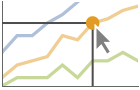
"Dropline" highlight and label the indicated point in a curve with droplines to the axes 
"XSlice" highlight and label all points along a vertical slice 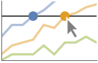
"YSlice" highlight and label all points along a horizontal slice 
Placed[effect,pos] statically highlight the given position pos - Highlight position specifications pos include:
-
x, {x} effect at {x,y} with y chosen automatically {x,y} effect at {x,y} {pos1,pos2,…} multiple positions posi
List of all options
Examples
open all close allBasic Examples (5)
Create a plot that stays level until the next date:
data = {{DateObject[{2006, 10, 1}, "Day", "Gregorian", -6.], 10}, {DateObject[{2006, 10, 15}, "Day", "Gregorian", -6.], 12}, {DateObject[{2006, 10, 30}, "Day", "Gregorian", -6.], 15}, {DateObject[{2006, 11, 20}, "Day", "Gregorian", -6.], 20}};DateListStepPlot[data]Draw the date points in the middle of the steps:
DateListStepPlot[data, Center, Mesh -> Full]Plot monthly values, starting in August 2000:
DateListStepPlot[{1, 2, 3, 4, 5, 6, 7}, {2000, 8}]Plot an individual component from a time series:
DateListStepPlot[TimeSeries[TimeEventSeries`TimestampData[Association["UniformlySpacedQ" -> True, "Count" -> 10,
   "Endpoints" -> TabularColumn[Association[
      "Data" -> {2, {{NumericArray[{15706, -2147483648}, "Integer32"], {},
          DataStructure["BitVe ... 7, 34, 40, 49, 54, 64, 72}, {}, None},
           "ElementType" -> "Integer64"]], TabularColumn[Association[
           "Data" -> {{1, 9, 11, 16, 18, 25, 34, 43, 49, 54}, {}, None},
           "ElementType" -> "Integer64"]]}}]]]], Association[]] -> "a", PlotLabels -> Automatic]
Plot multiple curves with a legend:
data1 = TimeSeries[{1, 1, 2, 3, 5, 8, 11}, {"Jan 1, 2015"}];
data2 = TimeSeries[{5, 8, 9, 6, 2, 4, 7}, {"Jan 1, 2015"}];DateListStepPlot[{data1, data2}, PlotLegends -> {"first", "second"}]DateListStepPlot[{data1, data2}, PlotLabels -> {"first", "second"}]Plot curves without the vertical segments:
DateListStepPlot[TemporalData[TimeSeries, {{{1, 1, 2, 3, 5, 8, 11}},
  {TemporalData`DateSpecification[{2015, 1, 1, 0, 0, 0.}, {2015, 1, 7, 0, 0, 0}, {1, "Day"}]}, 1,
  {"Continuous", 1}, {"Discrete", 1}, 1,
  {ResamplingMethod -> {"Interpolation", InterpolationOrder -> 1}}}, True, 314.1], Joined -> False]
Scope (49)
Data (13)
Steps are drawn through the date points:
data = {{DateObject[{2006, 10, 1}, "Day", "Gregorian", -6.], 10}, {DateObject[{2006, 10, 15}, "Day", "Gregorian", -6.], 12}, {DateObject[{2006, 10, 30}, "Day", "Gregorian", -6.], 15}, {DateObject[{2006, 11, 20}, "Day", "Gregorian", -6.], 20}};DateListStepPlot[data]DateListStepPlot[TemporalData[TimeSeries, {{{6.464000015258789, 6.367999992370605, 6.333333298012063,
6.5071428162711005, 6.407142843518939, 6.37333329518636, 6.466666645473904, 6.421052681772332,
6.427272666584361, 6.484615362607515, 6.285714285714286, 6 ... Data`DateSpecification[{2010, 1, 17, 20, 45, 32.},
{2013, 12, 17, 20, 45, 32}, {1, "Month"}]}, 1, {"Continuous", 1}, {"Discrete", 1}, 1,
{ValueDimensions -> 1, ResamplingMethod -> {"Interpolation", InterpolationOrder -> 1}}}, True,
10.3]]DateListStepPlot[TemporalData[EventSeries, {{{6.464000015258789, 6.367999992370605, 6.333333298012063,
6.5071428162711005, 6.407142843518939, 6.37333329518636, 6.466666645473904, 6.421052681772332,
6.427272666584361, 6.484615362607515, 6.285714285714286, ... 6.5,
6.199999809265137}}, {TemporalData`DateSpecification[{2010, 1, 17, 20, 45, 32.},
{2013, 12, 17, 20, 45, 32}, {1, "Month"}]}, 1, {"Continuous", 1}, {"Discrete", 1}, 1,
{ResamplingMethod -> None, ValueDimensions -> 1}}, True, 10.3]]Plot a series of data using an initial starting date or time:
DateListStepPlot[{2, 3, 5, 7, 11, 13, 17}, DateObject[{2015, 8, 15}, "Day", "Gregorian", -6.]]Plot data spaced equally in time between a starting and ending date:
DateListStepPlot[Sqrt[Range[10]], {DateObject[{2006, 5, 5}, "Day", "Gregorian", -6.], DateObject[{2006, 5, 30}, "Day", "Gregorian", -6.]}]Plot data gathered on the 15![]() day of each month, starting in January:
day of each month, starting in January:
DateListStepPlot[Range[5], {DateObject[{2006, 1, 15}, "Day", "Gregorian", -6.], Automatic, "Month"}]Dates given as DateString specifications:
DateListStepPlot[{{"June 2006", 10}, {"August 2006", 12}, {"November 2006", 15}, {"January 2007", 20}}]Use AbsoluteTime specifications:
DateListStepPlot[{{3368649600, 10}, {3369859200, 12}, {3371155200, 15}, {3372969600, 20}}]data1 = TemporalData[TimeSeries, {{{1, 1, 2, 3, 5, 8, 11}},
{TemporalData`DateSpecification[{2015, 1, 1, 0, 0, 0.}, {2015, 1, 7, 0, 0, 0}, {1, "Day"}]}, 1,
{"Continuous", 1}, {"Discrete", 1}, 1,
{ResamplingMethod -> {"Interpolation", InterpolationOrder -> 1}}}, True, 10.2];
data2 = TemporalData[TimeSeries, {{{5, 8, 9, 6, 2, 4, 7}},
{TemporalData`DateSpecification[{2015, 1, 1, 0, 0, 0.}, {2015, 1, 7, 0, 0, 0}, {1, "Day"}]}, 1,
{"Continuous", 1}, {"Discrete", 1}, 1,
{ResamplingMethod -> {"Interpolation", InterpolationOrder -> 1}}}, True, 10.2];DateListStepPlot[{data1, data2}]The plot range is selected automatically:
DateListStepPlot[TemporalData[TimeSeries, {{{6.464000015258789, 6.367999992370605, 6.333333298012063,
    6.5071428162711005, 6.407142843518939, 6.37333329518636, 6.466666645473904, 6.421052681772332,
    6.427272666584361, 6.484615362607515, 6.285714285714286, 6 ... Data`DateSpecification[{2010, 1, 17, 20, 45, 32.},
    {2013, 12, 17, 20, 45, 32}, {1, "Month"}]}, 1, {"Continuous", 1}, {"Discrete", 1}, 1,
  {ValueDimensions -> 1, ResamplingMethod -> {"Interpolation", InterpolationOrder -> 1}}}, True,
10.3]]Plot all the data in TimeSeries or EventSeries:
DateListStepPlot[TimeSeries[TimeEventSeries`TimestampData[Association["UniformlySpacedQ" -> False,
"Timestamps" -> TabularColumn[Association[
"Data" -> {7, {{NumericArray[{-248, 118, 298, 638, 865, 1006, 1216}, "Integer32"], {},
None}}, None}, ... "Data" -> {{32, 62, 112, 167, 179, 209, 214}, {}, None}, "ElementType" -> "Integer64"]],
TabularColumn[Association["Data" -> {{30, 49, 81, 125, 142, 174, 177}, {}, None},
"ElementType" -> "Integer64"]]}}]]]], Association[]]]Plot a specific component of a TimeSeries or EventSeries:
trees = TimeSeries[TimeEventSeries`TimestampData[Association["UniformlySpacedQ" -> False,
"Timestamps" -> TabularColumn[Association[
"Data" -> {7, {{NumericArray[{-248, 118, 298, 638, 865, 1006, 1216}, "Integer32"], {},
None}}, None}, ... "Data" -> {{32, 62, 112, 167, 179, 209, 214}, {}, None}, "ElementType" -> "Integer64"]],
TabularColumn[Association["Data" -> {{30, 49, 81, 125, 142, 174, 177}, {}, None},
"ElementType" -> "Integer64"]]}}]]]], Association[]];DateListStepPlot[trees -> "tree 1"]DateListStepPlot[trees -> {"tree 1", "tree 2"}]Use PlotRange to focus in on areas of interest:
DateListStepPlot[TemporalData[TimeSeries, {{{6.464000015258789, 6.367999992370605, 6.333333298012063,
6.5071428162711005, 6.407142843518939, 6.37333329518636, 6.466666645473904, 6.421052681772332,
6.427272666584361, 6.484615362607515, 6.285714285714286, 6 ... Data`DateSpecification[{2010, 1, 17, 20, 45, 32.},
{2013, 12, 17, 20, 45, 32}, {1, "Month"}]}, 1, {"Continuous", 1}, {"Discrete", 1}, 1,
{ValueDimensions -> 1, ResamplingMethod -> {"Interpolation", InterpolationOrder -> 1}}}, True,
10.3], PlotRange -> {{"Jan 1, 2011", "Dec 31, 2011"}, {6.2, 6.6}}]Use ScalingFunctions to scale the axes:
DateListStepPlot[{229, 627, 53, 1432, 931, 184}, Today, ScalingFunctions -> "Log"]Tabular Data (1)
Get tabular data for historical populations of several countries:
tab = Tabular[IconizedObject[«Country populations»]]Plot the population of France from 1940 to 2020:
DateListStepPlot[tab -> {"Date", "France"}]Plot the populations of France, Germany and Australia:
DateListStepPlot[tab -> {{"Date", "France"}, {"Date", "Germany"}, {"Date", "Australia"}}]Include legends for the plot, using the column names:
DateListStepPlot[tab -> {{"Date", "France"}, {"Date", "Germany"}, {"Date", "Australia"}}, PlotLegends -> {"France", "Germany", "Australia"}]Special Data (6)
Use Quantity to include units with the data:
DateListStepPlot[Quantity[Sqrt[Range[10]], "Meters"], {2010, 1, 1}, FrameLabel -> Automatic]Plot data in a QuantityArray:
qa = QuantityArray[RandomReal[{0, 40}, 20], "Fahrenheit"]DateListStepPlot[qa, {2000, 1, 1}, FrameLabel -> Automatic]Specify the units used with TargetUnits:
DateListStepPlot[qa, {2000, 1, 1}, TargetUnits -> "Kelvin", FrameLabel -> Automatic]Numeric values in an Association are used as the ![]() coordinates:
coordinates:
DateListStepPlot[<|"a" -> 2, "b" -> 3, "c" -> 5, "d" -> 7, "e" -> 11, "f" -> 13|>, "Jan, 1, 2010"]Numeric keys and values in an Association are used as the ![]() and
and ![]() coordinates:
coordinates:
DateListStepPlot[<|2 -> 1, 3 -> 2, 5 -> 3, 7 -> 4, 11 -> 5, 13 -> 6|>]Plot TimeSeries directly:
data = CountryData["UnitedStates", {{"Population"}, {1988, 2013}}]DateListStepPlot[data, FrameLabel -> Automatic]The weights in WeightedData are ignored:
DateListPlot[WeightedData[{2, 3, 5, 7, 11, 13, 17, 19, 23, 29}, {1, 2, 3, 4, 5, 6, 7, 8, 9, 10}], {2010, 1, 1}]Use a sparse array to represent the values:
DateListStepPlot[SparseArray[i_ /; PrimeQ[i] :> i, 20], DateObject[{2015, 7, 31}, "Day", "Gregorian", -6.]]Wrappers (8)
Use wrappers on individual data, datasets, or collections of datasets:
{DateListStepPlot[{Style[{1, 2, 3}, Green], {4, 5, 6}}, {2014, 8}], DateListStepPlot[Style[{{1, 2, 3}, {4, 5, 6}}, Blue], {2014, 8}]}DateListStepPlot[Style[{Style[{1, 2, 3}, Green], {4, 5, 6}}, Blue], {2014, 8}]Use the value of each point as a tooltip:
DateListStepPlot[Tooltip[Prime[Range[10]]], {2014, 8}, Center, Mesh -> Full]Use a specific label for all the points:
DateListStepPlot[Tooltip[Prime[Range[10]], "primes"], {2014, 8}, Center, Mesh -> Full]Use PopupWindow to provide additional drilldown information:
DateListStepPlot[{1, PopupWindow[2, DateListPlot[FinancialData["IBM", "Jan. 1, 2004"]]], 3}, {2004, 1}, Center, Mesh -> Full, PlotStyle -> PointSize[0.05]]Button can be used to trigger any action:
DateListStepPlot[{1, Button[2, Speak[2]], 3}, {2014, 8}, Center, Mesh -> Full, PlotStyle -> PointSize[0.05]]Use Annotation for dynamic action when the mouse enters the plot:
data = TemporalData[TimeSeries, {{{7, 12, 15, 20}}, {{{3368649600, 3369859200, 3371155200, 3372969600}}},
1, {"Continuous", 1}, {"Discrete", 1}, 1, {ValueDimensions -> 1, DateFunction -> Automatic,
ResamplingMethod -> {"Interpolation", InterpolationOrder -> 1}}}, True, 10.2];{DateListStepPlot[Annotation[data, "label", "Mouse"]], Dynamic[MouseAnnotation[]]}Use Hyperlink to jump to the specified link when clicked:
data = TemporalData[TimeSeries, {{{7, 12, 15, 20}}, {{{3368649600, 3369859200, 3371155200, 3372969600}}},
1, {"Continuous", 1}, {"Discrete", 1}, 1, {ValueDimensions -> 1, DateFunction -> Automatic,
ResamplingMethod -> {"Interpolation", InterpolationOrder -> 1}}}, True, 10.2];DateListStepPlot[Hyperlink[data, "http://www.wolfram.com"]]Use StatusArea to display a string in the status area of the current notebook:
data = TemporalData[TimeSeries, {{{7, 12, 15, 20}}, {{{3368649600, 3369859200, 3371155200, 3372969600}}},
1, {"Continuous", 1}, {"Discrete", 1}, 1, {ValueDimensions -> 1, DateFunction -> Automatic,
ResamplingMethod -> {"Interpolation", InterpolationOrder -> 1}}}, True, 10.2];DateListStepPlot[StatusArea[data, "String"]]Labeling and Legending (15)
Label data with Labeled:
data1 = Accumulate@RandomInteger[10, 10];data2 = Accumulate@RandomInteger[3, 10];DateListStepPlot[{Labeled[data1, "label1"], Labeled[data2, "label2"]}, {2010, 1, 1}]Label data with PlotLabels:
data1 = Accumulate@RandomInteger[10, 10];data2 = Accumulate@RandomInteger[3, 10];DateListStepPlot[{data1, data2}, {2000}, PlotLabels -> {"label1", "label2"}]Place the label near the points at an ![]() date:
date:
DateListStepPlot[Labeled[Accumulate@RandomInteger[10, 10], "label", {2004}], {2000}]DateListStepPlot[Labeled[Accumulate@RandomInteger[10, 10], "label", Scaled[0.3]], {2000}]Specify the text position relative to the point:
DateListStepPlot[Labeled[Accumulate@RandomInteger[10, 10], "label", {Scaled[0.3], Below}], {2000}]Label points with automatically positioned text:
DateListStepPlot[Table[Labeled[RandomReal[], i], {i, 15}], {2010, 1, 1}, PlotMarkers -> Automatic]Place the labels relative to the points:
Table[DateListStepPlot[Table[Labeled[RandomReal[], i, p], {i, 6}], {2010, 1, 1}, PlotMarkers -> Automatic, PlotLabel -> p], {p, {Above, Below, Before, After}}]Specify the maximum size of labels:
data = Rule[TimeSeries[{1, 1, 2, 3, 5, 8, 11}, {"Jan 1, 2015"}], RandomWord[7]];DateListStepPlot[data, LabelingSize -> 30]DateListStepPlot[data, LabelingSize -> Full]For dense sets of points, some labels may be turned into tooltips by default:
data = Rule[TimeSeries[RandomReal[1, 100], {"Jan 1, 2015"}], RandomWord[100]];DateListStepPlot[data, PlotMarkers -> Automatic]Increasing the size of the plot will show more labels:
DateListStepPlot[data, ImageSize -> 400, PlotMarkers -> Automatic]Label data automatically with Callout:
DateListStepPlot[{Callout[{2, 6, 10, 15, 15, 20, 24, 27, 27, 28}, "label1"], Callout[{1, 2, 3, 3, 4, 4, 4, 4, 5, 5}, "label2"]}, {2015, 1}]Place a label with a specific location:
DateListStepPlot[Callout[Table[n ^ Sin[n], {n, 1, 10, 0.25}], "label", Above], {2014, 1}]Include legends for each curve:
data1 = Accumulate@RandomInteger[10, 20];data2 = Accumulate@RandomInteger[3, 20];DateListStepPlot[{data1, data2}, {2000}, PlotLegends -> {"company1", "company2"}]Use Legended to provide a legend for a specific dataset:
data1 = Accumulate@RandomInteger[10, 20];data2 = Accumulate@RandomInteger[3, 20];DateListStepPlot[{data1, data2, Legended[data1 - data2, "difference"]}, {200}]Use Placed to change the legend location:
DateListStepPlot[{data1, data2, Legended[data1 - data2, Placed["difference", Bottom]]}, {200}]Use association keys as labels:
data1 = Accumulate@RandomInteger[10, 20];data2 = Accumulate@RandomInteger[3, 20];DateListStepPlot[<|"company A" -> data1, "company B" -> data2|>, {2000}, PlotLabels -> Automatic, PlotLegends -> None]Plots usually have interactive callouts showing the coordinates when you mouse over them:
DateListStepPlot[Range[15], {2007}]Including specific wrappers or interactions, such as tooltips, turns off the interactive features:
DateListStepPlot[Callout[Range[15], "hello", "01/01/2012"], {2007}]Use Highlighted to emphasize specific points in a plot:
DateListStepPlot[Highlighted[Range[15], Placed["Ball", DateObject[{2014, 1, 1}]]], {2007}]Use Highlighted[…,None] to disable highlighting for a single set:
DateListStepPlot[{Range[10], Highlighted[2 * Range[10], None]}, {2007}]Presentation (6)
Multiple curves are automatically colored to be distinct:
data1 = TemporalData[TimeSeries, {{{1, 1, 2, 3, 5, 8, 11}},
  {TemporalData`DateSpecification[{2015, 1, 1, 0, 0, 0.}, {2015, 1, 7, 0, 0, 0}, {1, "Day"}]}, 1,
  {"Continuous", 1}, {"Discrete", 1}, 1,
  {ResamplingMethod -> {"Interpolation", InterpolationOrder -> 1}}}, True, 10.2];
data2 = TemporalData[TimeSeries, {{{5, 8, 9, 6, 2, 4, 7}},
  {TemporalData`DateSpecification[{2015, 1, 1, 0, 0, 0.}, {2015, 1, 7, 0, 0, 0}, {1, "Day"}]}, 1,
  {"Continuous", 1}, {"Discrete", 1}, 1,
{ResamplingMethod -> {"Interpolation", InterpolationOrder -> 1}}}, True, 10.2];DateListStepPlot[{data1, data2}]Provide explicit styling to different curves:
DateListStepPlot[{data1, data2}, PlotStyle -> {Dashed, Red}]Include legends for each curve:
DateListStepPlot[{data1, data2}, PlotLegends -> {a, b}]Use Legended to provide a legend for a specific dataset:
DateListStepPlot[{Legended[data1, "data 1"], Legended[data2, "data 2"]}]Provide an interactive Tooltip for the curve:
data = TemporalData[TimeSeries, {{{7, 12, 15, 20}}, {{{3368649600, 3369859200, 3371155200, 3372969600}}},
1, {"Continuous", 1}, {"Discrete", 1}, 1, {ValueDimensions -> 1, DateFunction -> Automatic,
ResamplingMethod -> {"Interpolation", InterpolationOrder -> 1}}}, True, 314.1];DateListStepPlot[Tooltip[data, "Label"], Mesh -> Full]DateListStepPlot[Tooltip[{{DateObject[{2006, 10, 1}, TimeObject[{0, 0, 0.}, TimeZone -> -5.], TimeZone -> -5.], 7}, {DateObject[{2006, 10, 15}, TimeObject[{0, 0, 0.}, TimeZone -> -5.], TimeZone -> -5.], 12}, {DateObject[{2006, 10, 30}, TimeObject[{0, 0, 0.}, TimeZone -> -5.], TimeZone -> -5.], 15}, {DateObject[{2006, 11, 20}, TimeObject[{0, 0, 0.}, TimeZone -> -5.], TimeZone -> -5.], 20}}], Mesh -> Full]data1 = TemporalData[TimeSeries, {{{1, 1, 2, 3, 5, 8, 11}},
{TemporalData`DateSpecification[{2015, 1, 1, 0, 0, 0.}, {2015, 1, 7, 0, 0, 0}, {1, "Day"}]}, 1,
{"Continuous", 1}, {"Discrete", 1}, 1,
{ResamplingMethod -> {"Interpolation", InterpolationOrder -> 1}}}, True, 314.1];
data2 = TemporalData[TimeSeries, {{{5, 8, 9, 6, 2, 4, 7}},
{TemporalData`DateSpecification[{2015, 1, 1, 0, 0, 0.}, {2015, 1, 7, 0, 0, 0}, {1, "Day"}]}, 1,
{"Continuous", 1}, {"Discrete", 1}, 1,
{ResamplingMethod -> {"Interpolation", InterpolationOrder -> 1}}}, True, 314.1];DateListStepPlot[{data1, data2}, Filling -> Axis]Use shapes to distinguish different datasets:
DateListStepPlot[{TemporalData[...], TemporalData[...]}, Center, Mesh -> Full, PlotMarkers -> Automatic]Use a theme with simple ticks in a bold color scheme:
DateListStepPlot[{TemporalData[...], TemporalData[...]}, PlotTheme -> "Web"]Use a theme with bright colors on a dark background:
DateListStepPlot[{TemporalData[...], TemporalData[...]}, PlotTheme -> "Marketing"]Plot the data in a stacked layout:
data1 = {{DateObject[{2016, 10, 1}, "Day", "Gregorian", -5.], 10}, {DateObject[{2016, 10, 15}, "Day", "Gregorian", -5.], 17}, {DateObject[{2016, 10, 30}, "Day", "Gregorian", -5.], 15}, {DateObject[{2016, 11, 20}, "Day", "Gregorian", -5.], 20}};data2 = {{DateObject[{2016, 10, 1}, "Day", "Gregorian", -5.], 15}, {DateObject[{2016, 10, 15}, "Day", "Gregorian", -5.], 7}, {DateObject[{2016, 10, 30}, "Day", "Gregorian", -5.], 12}, {DateObject[{2016, 11, 20}, "Day", "Gregorian", -5.], 10}};DateListStepPlot[{data1, data2}, PlotLayout -> "Stacked"]Options (119)
AspectRatio (4)
By default, the ratio of the height to width for the plot is determined automatically:
DateListStepPlot[TemporalData[TimeSeries, {{{5, 8, 9, 6, 2, 4, 7}},
{TemporalData`DateSpecification[{2015, 1, 1, 0, 0, 0.}, {2015, 1, 7, 0, 0, 0}, {1, "Day"}]}, 1,
{"Continuous", 1}, {"Discrete", 1}, 1,
{ResamplingMethod -> {"Interpolation", InterpolationOrder -> 1}}}, True, 314.1]]Use a numerical value to specify the height-to-width ratio:
DateListStepPlot[TemporalData[TimeSeries, {{{5, 8, 9, 6, 2, 4, 7}},
{TemporalData`DateSpecification[{2015, 1, 1, 0, 0, 0.}, {2015, 1, 7, 0, 0, 0}, {1, "Day"}]}, 1,
{"Continuous", 1}, {"Discrete", 1}, 1,
{ResamplingMethod -> {"Interpolation", InterpolationOrder -> 1}}}, True, 314.1], AspectRatio -> 1 / 2]Make the height the same as the width with AspectRatio1:
DateListStepPlot[TemporalData[TimeSeries, {{{5, 8, 9, 6, 2, 4, 7}},
{TemporalData`DateSpecification[{2015, 1, 1, 0, 0, 0.}, {2015, 1, 7, 0, 0, 0}, {1, "Day"}]}, 1,
{"Continuous", 1}, {"Discrete", 1}, 1,
{ResamplingMethod -> {"Interpolation", InterpolationOrder -> 1}}}, True, 314.1], AspectRatio -> 1]AspectRatioFull adjusts the height and width to tightly fit inside other constructs:
plot = DateListStepPlot[TemporalData[TimeSeries, {{{5, 8, 9, 6, 2, 4, 7}},
{TemporalData`DateSpecification[{2015, 1, 1, 0, 0, 0.}, {2015, 1, 7, 0, 0, 0}, {1, "Day"}]}, 1,
{"Continuous", 1}, {"Discrete", 1}, 1,
{ResamplingMethod -> {"Interpolation", InterpolationOrder -> 1}}}, True, 314.1], AspectRatio -> Full];{Framed[Pane[plot, {50, 100}]], Framed[Pane[plot, {100, 100}]], Framed[Pane[plot, {100, 50}]]}Axes (1)
By default, DateListStepPlot uses a frame instead of axes:
data = TemporalData[TimeSeries, {{{1, 1, 2, 3, 5, 8, 11}},
{TemporalData`DateSpecification[{2015, 1, 1, 0, 0, 0.}, {2015, 1, 7, 0, 0, 0}, {1, "Day"}]}, 1,
{"Continuous", 1}, {"Discrete", 1}, 1,
{ResamplingMethod -> {"Interpolation", InterpolationOrder -> 1}}}, True, 10.2];DateListStepPlot[data]DateListStepPlot[data, Frame -> False, Axes -> True]DateListStepPlot[data, Frame -> False, Axes -> {True, False}]DateListStepPlot[data, Frame -> False, Axes -> {False, True}]AxesLabel (4)
No axes labels are drawn by default:
DateListStepPlot[TimeSeries[QuantityArray[Range[10], "Meters"], {"Jan 10,2021"}], Frame -> False, Axes -> True]DateListStepPlot[TimeSeries[QuantityArray[Range[10], "Meters"], {"Jan 10,2021"}], Frame -> False, Axes -> True, AxesLabel -> label]DateListStepPlot[TimeSeries[QuantityArray[Range[10], "Meters"], {"Jan 10,2021"}], Frame -> False, Axes -> True, AxesLabel -> {"Date", "Number"}]DateListStepPlot[TimeSeries[QuantityArray[Range[10], "Meters"], {"Jan 10,2021"}], Axes -> True, Frame -> False, AxesLabel -> Automatic]AxesOrigin (1)
The position of the axes is determined automatically:
DateListStepPlot[TemporalData[TimeSeries, {{{1, 1, 2, 3, 5, 8, 11}},
{TemporalData`DateSpecification[{2015, 8, 3, 0, 0, 0.}, {2015, 8, 9, 0, 0, 0}, {1, "Day"}]}, 1,
{"Continuous", 1}, {"Discrete", 1}, 1,
{ResamplingMethod -> {"Interpolation", InterpolationOrder -> 1}}}, True, 10.2], Frame -> False]Specify an explicit origin for the axes:
DateListStepPlot[TemporalData[TimeSeries, {{{1, 1, 2, 3, 5, 8, 11}},
{TemporalData`DateSpecification[{2015, 8, 3, 0, 0, 0.}, {2015, 8, 9, 0, 0, 0}, {1, "Day"}]}, 1,
{"Continuous", 1}, {"Discrete", 1}, 1,
{ResamplingMethod -> {"Interpolation", InterpolationOrder -> 1}}}, True, 10.2], Frame -> False, AxesOrigin -> {"August 1, 2015", 0}]AxesStyle (1)
Change the style for the axes:
data = TemporalData[TimeSeries, {{{1, 1, 2, 3, 5, 8, 11}},
{TemporalData`DateSpecification[{2015, 1, 1, 0, 0, 0.}, {2015, 1, 7, 0, 0, 0}, {1, "Day"}]}, 1,
{"Continuous", 1}, {"Discrete", 1}, 1,
{ResamplingMethod -> {"Interpolation", InterpolationOrder -> 1}}}, True, 10.2];DateListStepPlot[data, Frame -> False, Axes -> True, AxesStyle -> Red]Specify the style of each axis:
DateListStepPlot[data, Frame -> False, Axes -> True, AxesStyle -> {{Thick, Red}, {Thick, Blue}}]Use different styles for the ticks and the axes:
DateListStepPlot[data, Frame -> False, Axes -> True, AxesStyle -> Green, TicksStyle -> Red]Use different styles for the labels and the axes:
DateListStepPlot[data, Frame -> False, Axes -> True, AxesStyle -> Green, LabelStyle -> Red]ClippingStyle (1)
Omit clipped regions of the plot:
data = TemporalData[TimeSeries, {{{161.60000038146973, 159.19999980926514, 170.99999904632568,
91.09999942779541, 89.69999980926514, 95.59999942779541, 116.39999961853027,
122.00000095367432, 70.69999933242798, 84.2999997138977, 44., 85.09999990 ... Data`DateSpecification[{2010, 1, 17, 20, 45, 32.}, {2013, 12, 17, 20, 45, 32},
{1, "Month"}]}, 1, {"Continuous", 1}, {"Discrete", 1}, 1,
{ValueDimensions -> 1, ResamplingMethod -> {"Interpolation", InterpolationOrder -> 1}}}, True,
10.3];DateListStepPlot[data, ClippingStyle -> None]Show clipped regions as red at the bottom and the top:
DateListStepPlot[data, ClippingStyle -> Red]Use PlotRange->All to not clip:
DateListStepPlot[data, PlotRange -> All]ColorFunction (4)
Color with a named color scheme:
data = TemporalData[TimeSeries, {{{5, 8, 9, 6, 2, 4, 7}},
{TemporalData`DateSpecification[{2015, 1, 1, 0, 0, 0.}, {2015, 1, 7, 0, 0, 0}, {1, "Day"}]}, 1,
{"Continuous", 1}, {"Discrete", 1}, 1,
{ResamplingMethod -> {"Interpolation", InterpolationOrder -> 1}}}, True, 314.1];DateListStepPlot[data, ColorFunction -> "Rainbow"]Color by scaled ![]() and
and ![]() coordinates:
coordinates:
data = TemporalData[TimeSeries, {{{5, 8, 9, 6, 2, 4, 7}},
{TemporalData`DateSpecification[{2015, 1, 1, 0, 0, 0.}, {2015, 1, 7, 0, 0, 0}, {1, "Day"}]}, 1,
{"Continuous", 1}, {"Discrete", 1}, 1,
{ResamplingMethod -> {"Interpolation", InterpolationOrder -> 1}}}, True, 314.1];DateListStepPlot[data, ColorFunction -> Function[{x, y}, Hue[x]]]DateListStepPlot[data, ColorFunction -> Function[{x, y}, Hue[y]]]Fill with the color used for the curve:
data = TemporalData[TimeSeries, {{{5, 8, 9, 6, 2, 4, 7}},
{TemporalData`DateSpecification[{2015, 1, 1, 0, 0, 0.}, {2015, 1, 7, 0, 0, 0}, {1, "Day"}]}, 1,
{"Continuous", 1}, {"Discrete", 1}, 1,
{ResamplingMethod -> {"Interpolation", InterpolationOrder -> 1}}}, True, 314.1];DateListStepPlot[data, ColorFunction -> Function[{x, y}, Hue[x]], Filling -> Axis]ColorFunction has higher priority than PlotStyle for coloring the curve:
data = TemporalData[TimeSeries, {{{5, 8, 9, 6, 2, 4, 7}},
{TemporalData`DateSpecification[{2015, 1, 1, 0, 0, 0.}, {2015, 1, 7, 0, 0, 0}, {1, "Day"}]}, 1,
{"Continuous", 1}, {"Discrete", 1}, 1,
{ResamplingMethod -> {"Interpolation", InterpolationOrder -> 1}}}, True, 314.1];DateListStepPlot[data, ColorFunction -> "DarkRainbow", PlotStyle -> Directive[Red, Dashed]]ColorFunctionScaling (2)
Color the line based on scaled ![]() value:
value:
data = TemporalData[TimeSeries, {{{5, 8, 9, 6, 2, 4, 7}},
{TemporalData`DateSpecification[{2015, 1, 1, 0, 0, 0.}, {2015, 1, 7, 0, 0, 0}, {1, "Day"}]}, 1,
{"Continuous", 1}, {"Discrete", 1}, 1,
{ResamplingMethod -> {"Interpolation", InterpolationOrder -> 1}}}, True, 314.1];DateListStepPlot[data, ColorFunction -> Function[{x, y}, Hue[y]], PlotStyle -> Thick, ColorFunctionScaling -> True]Color the line based on unscaled ![]() value:
value:
data = TemporalData[TimeSeries, {{{5, 8, 9, 6, 2, 4, 7}},
{TemporalData`DateSpecification[{2015, 1, 1, 0, 0, 0.}, {2015, 1, 7, 0, 0, 0}, {1, "Day"}]}, 1,
{"Continuous", 1}, {"Discrete", 1}, 1,
{ResamplingMethod -> {"Interpolation", InterpolationOrder -> 1}}}, True, 314.1];DateListStepPlot[data, ColorFunction -> Function[{x, y}, Hue[y / 25]], PlotStyle -> Thick, ColorFunctionScaling -> False]DateFunction (1)
By default, numeric times correspond to AbsoluteTime:
data = {{100000000, 2}, {200000000, 3}, {300000000, 5}, {400000000, 7}, {500000000, 11}, {600000000, 13}, {700000000, 17}, {800000000, 19}, {900000000, 23}, {1000000000, 29}, {1100000000, 31}, {1200000000, 37}};DateListStepPlot[data]Interpret them as UnixTime:
DateListStepPlot[data, DateFunction -> FromUnixTime]DateTicksFormat (1)
Control how dates are formatted in labels:
data = TemporalData[TimeSeries, {{{10, 12, 15}}, {{{3.3607008*^9, 3.3645888*^9, 3.3663168*^9}}}, 1,
{"Continuous", 1}, {"Discrete", 1}, 1, {ValueDimensions -> 1, DateFunction -> Automatic,
ResamplingMethod -> {"Interpolation", InterpolationOrder -> 1}}}, True, 314.1];Table[DateListStepPlot[data, DateTicksFormat -> f], {f, {"MonthShort", "Month", "MonthNameShort", "MonthName"}}]Filling (2)
Explicitly specify the filling style for different plots:
data = TemporalData[TimeSeries, {{{5, 8, 9, 6, 2, 4, 7}},
{TemporalData`DateSpecification[{2015, 1, 1, 0, 0, 0.}, {2015, 1, 7, 0, 0, 0}, {1, "Day"}]}, 1,
{"Continuous", 1}, {"Discrete", 1}, 1,
{ResamplingMethod -> {"Interpolation", InterpolationOrder -> 1}}}, True, 314.1];Table[DateListStepPlot[data, Filling -> c], {c, {Top, Bottom, Axis, 5}}]Fills that overlap combine using opacity by default:
data1 = TemporalData[TimeSeries, {{{1, 1, 2, 3, 5, 8, 11}},
  {TemporalData`DateSpecification[{2015, 1, 1, 0, 0, 0.}, {2015, 1, 7, 0, 0, 0}, {1, "Day"}]}, 1,
  {"Continuous", 1}, {"Discrete", 1}, 1,
  {ResamplingMethod -> {"Interpolation", InterpolationOrder -> 1}}}, True, 10.2];
data2 = TemporalData[TimeSeries, {{{5, 8, 9, 6, 2, 4, 7}},
  {TemporalData`DateSpecification[{2015, 1, 1, 0, 0, 0.}, {2015, 1, 7, 0, 0, 0}, {1, "Day"}]}, 1,
  {"Continuous", 1}, {"Discrete", 1}, 1,
{ResamplingMethod -> {"Interpolation", InterpolationOrder -> 1}}}, True, 10.2];DateListStepPlot[{data1, data2}, Filling -> Axis]Fill from the second curve to the first:
DateListStepPlot[{data1, data2}, Filling -> {2 -> {1}}]Fill the region between two curves with light gray:
DateListStepPlot[{data1, data2}, Filling -> {2 -> {{1}, LightGray}}]FillingStyle (3)
data = TemporalData[TimeSeries, {{{1, 1, 2, 3, 5, 8, 11}},
{TemporalData`DateSpecification[{2015, 1, 1, 0, 0, 0.}, {2015, 1, 7, 0, 0, 0}, {1, "Day"}]}, 1,
{"Continuous", 1}, {"Discrete", 1}, 1,
{ResamplingMethod -> {"Interpolation", InterpolationOrder -> 1}}}, True, 10.2];DateListStepPlot[data, Filling -> Axis, FillingStyle -> Red]Fill with red below the axis and with blue above:
DateListStepPlot[data, Filling -> Axis, FillingStyle -> {Red, Blue}]data1 = TemporalData[TimeSeries, {{{1, 1, 2, 3, 5, 8, 11}},
{TemporalData`DateSpecification[{2015, 1, 1, 0, 0, 0.}, {2015, 1, 7, 0, 0, 0}, {1, "Day"}]}, 1,
{"Continuous", 1}, {"Discrete", 1}, 1,
{ResamplingMethod -> {"Interpolation", InterpolationOrder -> 1}}}, True, 10.2];
data2 = TemporalData[TimeSeries, {{{5, 8, 9, 6, 2, 4, 7}},
{TemporalData`DateSpecification[{2015, 1, 1, 0, 0, 0.}, {2015, 1, 7, 0, 0, 0}, {1, "Day"}]}, 1,
{"Continuous", 1}, {"Discrete", 1}, 1,
{ResamplingMethod -> {"Interpolation", InterpolationOrder -> 1}}}, True, 10.2];DateListStepPlot[{data1, data2}, Filling -> Axis, FillingStyle -> Directive[Opacity[0.5], Orange]]Use a variable filling style obtained from ColorFunction:
data = TemporalData[TimeSeries, {{{1, 1, 2, 3, 5, 8, 11}},
{TemporalData`DateSpecification[{2015, 8, 1, 0, 0, 0.}, {2015, 8, 7, 0, 0, 0}, {1, "Day"}]}, 1,
{"Continuous", 1}, {"Discrete", 1}, 1,
{ResamplingMethod -> {"Interpolation", InterpolationOrder -> 1}}}, True, 10.2];DateListStepPlot[data, ColorFunction -> Function[{x, y}, Hue[y]], Filling -> Axis, FillingStyle -> Automatic]Frame (4)
DateListStepPlot uses a frame by default:
DateListStepPlot[Range[10], {2007}]Use FrameFalse to turn off the frame:
DateListStepPlot[Range[10], {2007}, Frame -> False]Draw a frame on the left and right edges:
DateListStepPlot[Range[10], {2007}, Frame -> {{True, True}, {False, False}}]Draw a frame on the left and bottom edges:
DateListStepPlot[Range[10], {2007}, Frame -> {{True, False}, {True, False}}]FrameLabel (4)
Place a label along the bottom frame of a plot:
DateListStepPlot[Range[10], {2007}, FrameLabel -> {"label"}]Frame labels are placed on the bottom and left frame edges by default:
DateListStepPlot[Range[10], {2007}, FrameLabel -> {"Bottom", "Left"}]Place labels on each of the edges in the frame:
DateListStepPlot[Range[10], {2007}, FrameLabel -> {{"left", "right"}, {"bottom", "top"}}]Use a customized style for both labels and frame tick labels:
DateListStepPlot[Range[10], {2007}, FrameLabel -> {{"left", "right"}, {"bottom", "top"}}, LabelStyle -> Directive[Bold, StandardGreen]]FrameStyle (2)
Specify the style of the frame:
DateListStepPlot[Range[10], {2007}, FrameStyle -> Directive[StandardGreen, Thick]]Specify the style for each frame edge:
DateListStepPlot[Range[10], {2007}, FrameStyle -> {{Directive[StandardGreen, Thick], Directive[Red, Thick]}, {Directive[Gray, Thick], Directive[Blue, Thick]}}]FrameTicks (9)
Frame ticks are placed automatically by default:
DateListStepPlot[Range[10], {2007}]DateListStepPlot[Range[10], {2007}, FrameTicks -> None]Use frame ticks on the bottom edge:
DateListStepPlot[Range[10], {2007}, FrameTicks -> {{None, None}, {Automatic, None}}]By default, the top and right edges have tick marks but no tick labels:
DateListStepPlot[Range[10], {2007}, FrameTicks -> Automatic]Use All to include tick labels on all edges:
DateListStepPlot[Range[10], {2007}, FrameTicks -> All]Place tick marks at specific positions:
DateListStepPlot[Range[10], {2007}, FrameTicks -> {{{2, .5, 10}, None}, {{"July 1, 2011", "July 1, 2014"}, None}}]Draw frame tick marks at the specified positions with specific labels:
DateListStepPlot[Range[10], {2007}, FrameTicks -> {{{{2, "two"}, {5, "five"}, {10, "ten"}}, None}, {{{"July 1, 2011", "date 1"}, {"July 1, 2014", "date 2"}}, None}}]Specify the lengths for tick marks as a fraction of the graphics size:
DateListStepPlot[Range[10], {2007}, FrameTicks -> {{{{2, "two", .15}, {5, "five", .45}, {10, "ten", .95}}, None}, {Automatic, None}}]Use different sizes in the positive and negative directions for each tick mark:
DateListStepPlot[Range[10], {2007}, FrameTicks -> {{{{2, "two", {.15, .1}}, {5, "five", {.45, .2}}, {10, "ten", {.95, .3}}}, None}, {Automatic, None}}]Specify a style for each frame tick:
DateListStepPlot[Range[10], {2007}, FrameTicks -> {{{{2, "two", .12, Directive[Blue, Thick]}, {5, "five", .4, Directive[Red, Thick, Dashed]}, {10, "ten", .9, Directive[Green, Thick, Dashed]}}, None}, {Automatic, None}}]Construct a function that places frame ticks at the midpoint and extremes of the frame edge:
minMeanMax[min_, max_] := {{min, min}, {(max + min) / 2, (max + min) / 2}, {max, max}}DateListStepPlot[Range[10], {2007}, FrameTicks -> {{minMeanMax, None}, {Automatic, None}}, PlotRangePadding -> None]FrameTicksStyle (3)
By default, the frame ticks and frame tick labels use the same styles as the frame:
DateListStepPlot[Range[10], {2007}, FrameStyle -> Directive[Red]]Specify an overall style for the ticks, including the labels:
DateListStepPlot[Range[10], {2007}, FrameStyle -> Directive[Red], FrameTicksStyle -> Directive[Blue, Thick]]Use different styles for the different frame edges:
DateListStepPlot[Range[10], {2007}, FrameTicks -> All, FrameTicksStyle -> {{Directive[Orange, Thick], Blue}, {Red, Green}}]GridLines (1)
data = TemporalData[TimeSeries, {{{1, 1, 2, 3, 5, 8, 11}},
{TemporalData`DateSpecification[{2015, 8, 1, 0, 0, 0.}, {2015, 8, 7, 0, 0, 0}, {1, "Day"}]}, 1,
{"Continuous", 1}, {"Discrete", 1}, 1,
{ResamplingMethod -> {"Interpolation", InterpolationOrder -> 1}}}, True, 10.2];DateListStepPlot[data, GridLines -> Automatic]Draw grid lines at the specific positions:
DateListStepPlot[data, GridLines -> {{"Aug 2, 2015", "Aug 6, 2015"}, None}]GridLinesStyle (1)
data = TemporalData[TimeSeries, {{{1, 1, 2, 3, 5, 8, 11}},
{TemporalData`DateSpecification[{2015, 1, 1, 0, 0, 0.}, {2015, 1, 7, 0, 0, 0}, {1, "Day"}]}, 1,
{"Continuous", 1}, {"Discrete", 1}, 1,
{ResamplingMethod -> {"Interpolation", InterpolationOrder -> 1}}}, True, 314.1];DateListStepPlot[data, GridLines -> Automatic, GridLinesStyle -> Dotted]ImageSize (7)
Use named sizes such as Tiny, Small, Medium and Large:
{DateListStepPlot[TemporalData[TimeSeries, {{{5, 8, 9, 6, 2, 4, 7}},
{TemporalData`DateSpecification[{2015, 1, 1, 0, 0, 0.}, {2015, 1, 7, 0, 0, 0}, {1, "Day"}]}, 1,
{"Continuous", 1}, {"Discrete", 1}, 1,
{ResamplingMethod -> {"Interpolation", InterpolationOrder -> 1}}}, True, 314.1], ImageSize -> Tiny], DateListStepPlot[TemporalData[TimeSeries, {{{5, 8, 9, 6, 2, 4, 7}},
{TemporalData`DateSpecification[{2015, 1, 1, 0, 0, 0.}, {2015, 1, 7, 0, 0, 0}, {1, "Day"}]}, 1,
{"Continuous", 1}, {"Discrete", 1}, 1,
{ResamplingMethod -> {"Interpolation", InterpolationOrder -> 1}}}, True, 314.1], ImageSize -> Small]}Specify the width of the plot:
{DateListStepPlot[TemporalData[TimeSeries, {{{5, 8, 9, 6, 2, 4, 7}},
{TemporalData`DateSpecification[{2015, 1, 1, 0, 0, 0.}, {2015, 1, 7, 0, 0, 0}, {1, "Day"}]}, 1,
{"Continuous", 1}, {"Discrete", 1}, 1,
{ResamplingMethod -> {"Interpolation", InterpolationOrder -> 1}}}, True, 314.1], ImageSize -> 150], DateListStepPlot[TemporalData[TimeSeries, {{{5, 8, 9, 6, 2, 4, 7}},
{TemporalData`DateSpecification[{2015, 1, 1, 0, 0, 0.}, {2015, 1, 7, 0, 0, 0}, {1, "Day"}]}, 1,
{"Continuous", 1}, {"Discrete", 1}, 1,
{ResamplingMethod -> {"Interpolation", InterpolationOrder -> 1}}}, True, 314.1], AspectRatio -> 1.5, ImageSize -> 150]}Specify the height of the plot:
{DateListStepPlot[TemporalData[TimeSeries, {{{5, 8, 9, 6, 2, 4, 7}},
{TemporalData`DateSpecification[{2015, 1, 1, 0, 0, 0.}, {2015, 1, 7, 0, 0, 0}, {1, "Day"}]}, 1,
{"Continuous", 1}, {"Discrete", 1}, 1,
{ResamplingMethod -> {"Interpolation", InterpolationOrder -> 1}}}, True, 314.1], ImageSize -> {Automatic, 150}], DateListStepPlot[TemporalData[TimeSeries, {{{5, 8, 9, 6, 2, 4, 7}},
{TemporalData`DateSpecification[{2015, 1, 1, 0, 0, 0.}, {2015, 1, 7, 0, 0, 0}, {1, "Day"}]}, 1,
{"Continuous", 1}, {"Discrete", 1}, 1,
{ResamplingMethod -> {"Interpolation", InterpolationOrder -> 1}}}, True, 314.1], AspectRatio -> 2, ImageSize -> {Automatic, 150}]}Allow the width and height to be up to a certain size:
{DateListStepPlot[TemporalData[TimeSeries, {{{5, 8, 9, 6, 2, 4, 7}},
{TemporalData`DateSpecification[{2015, 1, 1, 0, 0, 0.}, {2015, 1, 7, 0, 0, 0}, {1, "Day"}]}, 1,
{"Continuous", 1}, {"Discrete", 1}, 1,
{ResamplingMethod -> {"Interpolation", InterpolationOrder -> 1}}}, True, 314.1], ImageSize -> UpTo[200]], DateListStepPlot[TemporalData[TimeSeries, {{{5, 8, 9, 6, 2, 4, 7}},
{TemporalData`DateSpecification[{2015, 1, 1, 0, 0, 0.}, {2015, 1, 7, 0, 0, 0}, {1, "Day"}]}, 1,
{"Continuous", 1}, {"Discrete", 1}, 1,
{ResamplingMethod -> {"Interpolation", InterpolationOrder -> 1}}}, True, 314.1], AspectRatio -> 2, ImageSize -> UpTo[200]]}Specify the width and height for a graphic, padding with space if necessary:
DateListStepPlot[TemporalData[TimeSeries, {{{5, 8, 9, 6, 2, 4, 7}},
{TemporalData`DateSpecification[{2015, 1, 1, 0, 0, 0.}, {2015, 1, 7, 0, 0, 0}, {1, "Day"}]}, 1,
{"Continuous", 1}, {"Discrete", 1}, 1,
{ResamplingMethod -> {"Interpolation", InterpolationOrder -> 1}}}, True, 314.1], ImageSize -> {200, 200}, Background -> StandardGray]Setting AspectRatioFull will fill the available space:
DateListStepPlot[TemporalData[TimeSeries, {{{5, 8, 9, 6, 2, 4, 7}},
{TemporalData`DateSpecification[{2015, 1, 1, 0, 0, 0.}, {2015, 1, 7, 0, 0, 0}, {1, "Day"}]}, 1,
{"Continuous", 1}, {"Discrete", 1}, 1,
{ResamplingMethod -> {"Interpolation", InterpolationOrder -> 1}}}, True, 314.1], AspectRatio -> Full, ImageSize -> {200, 200}, Background -> StandardGray]Use maximum sizes for the width and height:
{DateListStepPlot[TemporalData[TimeSeries, {{{5, 8, 9, 6, 2, 4, 7}},
{TemporalData`DateSpecification[{2015, 1, 1, 0, 0, 0.}, {2015, 1, 7, 0, 0, 0}, {1, "Day"}]}, 1,
{"Continuous", 1}, {"Discrete", 1}, 1,
{ResamplingMethod -> {"Interpolation", InterpolationOrder -> 1}}}, True, 314.1], ImageSize -> {UpTo[150], UpTo[100]}], DateListStepPlot[TemporalData[TimeSeries, {{{5, 8, 9, 6, 2, 4, 7}},
{TemporalData`DateSpecification[{2015, 1, 1, 0, 0, 0.}, {2015, 1, 7, 0, 0, 0}, {1, "Day"}]}, 1,
{"Continuous", 1}, {"Discrete", 1}, 1,
{ResamplingMethod -> {"Interpolation", InterpolationOrder -> 1}}}, True, 314.1], AspectRatio -> 2, ImageSize -> {UpTo[150], UpTo[100]}]}Use ImageSizeFull to fill the available space in an object:
Framed[Pane[DateListStepPlot[TemporalData[TimeSeries, {{{5, 8, 9, 6, 2, 4, 7}},
{TemporalData`DateSpecification[{2015, 1, 1, 0, 0, 0.}, {2015, 1, 7, 0, 0, 0}, {1, "Day"}]}, 1,
{"Continuous", 1}, {"Discrete", 1}, 1,
{ResamplingMethod -> {"Interpolation", InterpolationOrder -> 1}}}, True, 314.1], ImageSize -> Full, Background -> StandardGray], {200, 100}]]Specify the image size as a fraction of the available space:
Framed[Pane[DateListStepPlot[TemporalData[TimeSeries, {{{5, 8, 9, 6, 2, 4, 7}},
{TemporalData`DateSpecification[{2015, 1, 1, 0, 0, 0.}, {2015, 1, 7, 0, 0, 0}, {1, "Day"}]}, 1,
{"Continuous", 1}, {"Discrete", 1}, 1,
{ResamplingMethod -> {"Interpolation", InterpolationOrder -> 1}}}, True, 314.1], ImageSize -> {Scaled[0.5], Scaled[0.5]}, Background -> StandardGray], {200, 100}]]Joined (1)
By default, the horizontal steps are joined by vertical segments:
data = TemporalData[TimeSeries, {{{1, 1, 2, 3, 5, 8, 11}},
{TemporalData`DateSpecification[{2015, 1, 1, 0, 0, 0.}, {2015, 1, 7, 0, 0, 0}, {1, "Day"}]}, 1,
{"Continuous", 1}, {"Discrete", 1}, 1,
{ResamplingMethod -> {"Interpolation", InterpolationOrder -> 1}}}, True, 314.1];DateListStepPlot[data]Use Joined->False to create a plot without the vertical segments:
DateListStepPlot[data, Joined -> False]LabelingSize (4)
Textual labels are shown at their actual sizes:
DateListPlot[TimeSeries[{1, 1, 2, 3, 5, 8}, {"Jan 1, 2015"}] -> {"healthfulness", "obstreperous", "spectrogram", "vestige", "coinage", "limey"}, ImageSize -> Medium]Image labels are automatically resized:
DateListStepPlot[TimeSeries[{1, 1, 2, 3, 5, 8}, {"Jan 1, 2015"}] -> {[image], [image], [image], [image], [image], [image]}, ImageSize -> Medium]Specify a maximum size for textual labels:
DateListStepPlot[TimeSeries[{1, 1, 2, 3, 5, 8}, {"Jan 1, 2015"}] -> {"healthfulness", "obstreperous", "spectrogram", "vestige", "coinage", "limey"}, ImageSize -> Medium, LabelingSize -> 30]Specify a maximum size for image labels:
DateListStepPlot[TimeSeries[{1, 1, 2, 3, 5, 8}, {"Jan 1, 2015"}] -> {[image], [image], [image], [image], [image], [image]}, ImageSize -> Medium, LabelingSize -> 20]Show image labels at their natural sizes:
DateListStepPlot[TimeSeries[{1, 1, 2, 3, 5, 8}, {"Jan 1, 2015"}] -> {[image], [image], [image], [image], [image], [image]}, ImageSize -> Medium, LabelingSize -> Full]Mesh (1)
Use Mesh->Full to show the point for each step:
data = TemporalData[TimeSeries, {{{1, 1, 2, 3, 5, 8, 11}},
{TemporalData`DateSpecification[{2015, 1, 1, 0, 0, 0.}, {2015, 1, 7, 0, 0, 0}, {1, "Day"}]}, 1,
{"Continuous", 1}, {"Discrete", 1}, 1,
{ResamplingMethod -> {"Interpolation", InterpolationOrder -> 1}}}, True, 314.1];DateListStepPlot[data, Mesh -> Full]Table[DateListStepPlot[data, step, Mesh -> Full, PlotLabel -> step], {step, {Left, Right, Center}}]Use different mesh specifications:
Table[DateListStepPlot[data, Mesh -> m, PlotLabel -> Mesh -> m], {m, {All, 15, None, Automatic}}]MeshFunctions (1)
Show seven mesh levels in the ![]() direction (red) and 10 mesh levels in the
direction (red) and 10 mesh levels in the ![]() direction (blue):
direction (blue):
data = TemporalData[TimeSeries, {{{1, 1, 2, 3, 5, 8, 11}},
{TemporalData`DateSpecification[{2015, 8, 1, 0, 0, 0.}, {2015, 8, 7, 0, 0, 0}, {1, "Day"}]}, 1,
{"Continuous", 1}, {"Discrete", 1}, 1,
{ResamplingMethod -> {"Interpolation", InterpolationOrder -> 1}}}, True, 10.2];DateListStepPlot[data, Center, Mesh -> {7, 10}, MeshFunctions -> {#1&, #2&}, MeshStyle -> {Directive[PointSize[Medium], Red], Blue}]MeshShading (1)
Alternate red and blue segments of equal width in the ![]() direction:
direction:
data = TemporalData[TimeSeries, {{{1, 1, 2, 3, 5, 8, 11}},
{TemporalData`DateSpecification[{2015, 1, 1, 0, 0, 0.}, {2015, 1, 7, 0, 0, 0}, {1, "Day"}]}, 1,
{"Continuous", 1}, {"Discrete", 1}, 1,
{ResamplingMethod -> {"Interpolation", InterpolationOrder -> 1}}}, True, 314.1];DateListStepPlot[data, Mesh -> 15, MeshFunctions -> {#1&}, MeshShading -> {Red, Blue}]MeshShading can be used with PlotStyle:
DateListStepPlot[data, Mesh -> 15, PlotStyle -> Dashed, MeshFunctions -> {#1&}, MeshShading -> {Red, Blue}]MeshStyle (1)
Use different mesh directives:
data = TemporalData[TimeSeries, {{{1, 1, 2, 3, 5, 8, 11}},
{TemporalData`DateSpecification[{2015, 8, 1, 0, 0, 0.}, {2015, 8, 7, 0, 0, 0}, {1, "Day"}]}, 1,
{"Continuous", 1}, {"Discrete", 1}, 1,
{ResamplingMethod -> {"Interpolation", InterpolationOrder -> 1}}}, True, 10.2];DateListStepPlot[data, Mesh -> Full, MeshStyle -> Red]PlotFit (4)
Automatically fit a model to the data:
DateListStepPlot[TimeSeries[TimeEventSeries`TimestampData[Association["UniformlySpacedQ" -> False,
"Timestamps" -> TabularColumn[Association[
"Data" -> {61, {{NumericArray[{19724, 19725, 19726, 19727, 19730, 19731, 19732, 19733, 19734,
19738, ... 94.28900146484375, 95.00199890136719, 92.56099700927734, 90.25, 90.35600280761719}, {},
None}}, None}, "ElementType" -> TypeSpecifier["Quantity"]["Real64", "USDollars"]]],
Association["ResamplingMethod" -> "LinearInterpolation"]], PlotFit -> Automatic]Fit a straight line to the data:
DateListStepPlot[TimeSeries[TimeEventSeries`TimestampData[Association["UniformlySpacedQ" -> False,
"Timestamps" -> TabularColumn[Association[
"Data" -> {61, {{NumericArray[{19724, 19725, 19726, 19727, 19730, 19731, 19732, 19733, 19734,
19738, ... 94.28900146484375, 95.00199890136719, 92.56099700927734, 90.25, 90.35600280761719}, {},
None}}, None}, "ElementType" -> TypeSpecifier["Quantity"]["Real64", "USDollars"]]],
Association["ResamplingMethod" -> "LinearInterpolation"]], PlotFit -> "Linear"]Fit a quadratic curve to the data:
DateListStepPlot[TimeSeries[TimeEventSeries`TimestampData[Association["UniformlySpacedQ" -> False,
"Timestamps" -> TabularColumn[Association[
"Data" -> {61, {{NumericArray[{19724, 19725, 19726, 19727, 19730, 19731, 19732, 19733, 19734,
19738, ... 94.28900146484375, 95.00199890136719, 92.56099700927734, 90.25, 90.35600280761719}, {},
None}}, None}, "ElementType" -> TypeSpecifier["Quantity"]["Real64", "USDollars"]]],
Association["ResamplingMethod" -> "LinearInterpolation"]], PlotFit -> "Quadratic"]Fit a periodic model to the data:
DateListStepPlot[TimeSeries[TimeEventSeries`TimestampData[Association["UniformlySpacedQ" -> False,
"Timestamps" -> TabularColumn[Association[
"Data" -> {61, {{NumericArray[{19724, 19725, 19726, 19727, 19730, 19731, 19732, 19733, 19734,
19738, ... 94.28900146484375, 95.00199890136719, 92.56099700927734, 90.25, 90.35600280761719}, {},
None}}, None}, "ElementType" -> TypeSpecifier["Quantity"]["Real64", "USDollars"]]],
Association["ResamplingMethod" -> "LinearInterpolation"]], PlotFit -> PeriodicModel[3]]//QuietPlotFitElements (2)
Plot confidence bands for the data, with a default confidence level of 0.95:
DateListStepPlot[TimeSeries[TimeEventSeries`TimestampData[Association["UniformlySpacedQ" -> False,
"Timestamps" -> TabularColumn[Association[
"Data" -> {61, {{NumericArray[{19724, 19725, 19726, 19727, 19730, 19731, 19732, 19733, 19734,
19738, ... 94.28900146484375, 95.00199890136719, 92.56099700927734, 90.25, 90.35600280761719}, {},
None}}, None}, "ElementType" -> TypeSpecifier["Quantity"]["Real64", "USDollars"]]],
Association["ResamplingMethod" -> "LinearInterpolation"]], PlotFit -> Automatic, PlotFitElements -> "BandCurves"]Use a confidence level of 0.5 for the bands:
DateListStepPlot[TimeSeries[TimeEventSeries`TimestampData[Association["UniformlySpacedQ" -> False,
"Timestamps" -> TabularColumn[Association[
"Data" -> {61, {{NumericArray[{19724, 19725, 19726, 19727, 19730, 19731, 19732, 19733, 19734,
19738, ... 94.28900146484375, 95.00199890136719, 92.56099700927734, 90.25, 90.35600280761719}, {},
None}}, None}, "ElementType" -> TypeSpecifier["Quantity"]["Real64", "USDollars"]]],
Association["ResamplingMethod" -> "LinearInterpolation"]], PlotFit -> Automatic, PlotFitElements -> {"BandCurves", <|"ConfidenceLevel" -> 0.5|>}]Show residual lines from the data points to the fitted curve:
DateListStepPlot[TimeSeries[TimeEventSeries`TimestampData[Association["UniformlySpacedQ" -> False,
"Timestamps" -> TabularColumn[Association[
"Data" -> {61, {{NumericArray[{19724, 19725, 19726, 19727, 19730, 19731, 19732, 19733, 19734,
19738, ... 94.28900146484375, 95.00199890136719, 92.56099700927734, 90.25, 90.35600280761719}, {},
None}}, None}, "ElementType" -> TypeSpecifier["Quantity"]["Real64", "USDollars"]]],
Association["ResamplingMethod" -> "LinearInterpolation"]], PlotFit -> Automatic, PlotFitElements -> "Residuals"]Combine the original points with gray residual lines:
DateListStepPlot[TimeSeries[TimeEventSeries`TimestampData[Association["UniformlySpacedQ" -> False,
"Timestamps" -> TabularColumn[Association[
"Data" -> {61, {{NumericArray[{19724, 19725, 19726, 19727, 19730, 19731, 19732, 19733, 19734,
19738, ... 94.28900146484375, 95.00199890136719, 92.56099700927734, 90.25, 90.35600280761719}, {},
None}}, None}, "ElementType" -> TypeSpecifier["Quantity"]["Real64", "USDollars"]]],
Association["ResamplingMethod" -> "LinearInterpolation"]], PlotFit -> Automatic, PlotFitElements -> {"DataPoints", {"Residuals", <|"Style" -> Opacity[1, StandardRed]|>}}]PlotHighlighting (9)
Plots have interactive coordinate callouts with the default setting PlotHighlightingAutomatic:
DateListStepPlot[Range[10], {2007}]Use PlotHighlightingNone to disable the highlighting for the entire plot:
DateListStepPlot[Range[10], {2007}, PlotHighlighting -> None]Move the mouse over a set of points to highlight it using arbitrary graphics directives:
DateListPlot[{Range[10], 2 * Range[10]}, {2007}, PlotHighlighting -> Directive[Red, AbsolutePointSize[10], DropShadowing[]]]Move the mouse over the points to highlight them with balls and labels:
DateListStepPlot[{Range[10], 2 * Range[10]}, {2007}, PlotHighlighting -> "Dropline"]Move the mouse over the curve to highlight it with a label and drop lines to the axes:
DateListStepPlot[Range[10], {2007}, PlotHighlighting -> "Dropline"]Use a ball and label to highlight a specific point in the plot:
DateListStepPlot[Range[10], {2007}, PlotHighlighting -> Placed["Dropline", DateObject[{2012, 1, 1}]]]Move the mouse over the plot to highlight it with a slice showing ![]() values corresponding to the
values corresponding to the ![]() position:
position:
DateListStepPlot[{Range[10], 2 * Range[10]}, {2007}, PlotHighlighting -> "XSlice"]Highlight a particular set of points at a fixed ![]() value:
value:
DateListStepPlot[Range[10], {2007}, PlotHighlighting -> Placed["XSlice", DateObject[{2014, 1, 1}]]]Move the mouse over the plot to highlight it with a slice showing ![]() values corresponding to the
values corresponding to the ![]() position:
position:
DateListStepPlot[{Range[10], 2 * Range[10]}, {2007}, PlotHighlighting -> "YSlice"]Highlight the curves at a fixed ![]() value:
value:
DateListStepPlot[{Range[10], 2 * Range[10]}, {2007}, PlotHighlighting -> Placed["YSlice", 4]]Use a component that shows the points on the plot closest to the ![]() position of the mouse cursor:
position of the mouse cursor:
DateListStepPlot[{Range[10], 2 * Range[10]}, {2007}, PlotHighlighting -> "XNearestPoint"]Specify the style for the points:
DateListStepPlot[{Range[10], 2 * Range[10]}, {2007}, PlotHighlighting -> {"XNearestPoint", <|"Style" -> StandardGray|>}]Use a component that shows the coordinates on the points closest to the mouse cursor:
DateListStepPlot[{Range[10], 2 * Range[10]}, {2007}, PlotHighlighting -> "XYLabel"]Use Callout options to change the appearance of the label:
DateListStepPlot[{Range[10], 2 * Range[10]}, {2007}, PlotHighlighting -> {"XYLabel", <|"Appearance" -> "Corners", "CalloutMarker" -> "Circle"|>}]Combine components to create a custom effect:
DateListStepPlot[{Range[10], 2 * Range[10]}, {2007}, PlotHighlighting -> {{"XNearestPoint", <|"Style" -> StandardGray|>}, {"XYLabel", <|"Appearance" -> "Corners", "CalloutMarker" -> "Circle"|>}}]DateListStepPlot[{Range[10], 2 * Range[10]}, {2007}, PlotHighlighting -> {"XYLabel", <|"NumberForm" -> 4, "LabelingFunction" -> (Grid[{{"x", First[#1]}, {"y", Last[#1]}}]&)|>}]PlotInteractivity (3)
Plots have interactive highlighting by default:
DateListStepPlot[{2, 3, 5, 7, 11, 13, 17, 19, 23, 29}, Today]Turn off all the interactive elements:
DateListStepPlot[{2, 3, 5, 7, 11, 13, 17, 19, 23, 29}, Today, PlotInteractivity -> False]Allow provided interactive elements and disable automatic ones:
DateListStepPlot[{2, 3, 5, 7, 11, 13, 17, 19, 23, Tooltip[29, "hello"]}, Today, PlotMarkers -> Automatic, PlotInteractivity -> <|"User" -> True, "System" -> False|>]PlotLabel (1)
PlotLabels (4)
data1 = Transpose[{DateRange[{2000, 1, 1}, {2000, 1, 15}], RandomReal[10, 15]}];data2 = Transpose[{DateRange[{2000, 1, 1}, {2000, 1, 15}], RandomReal[10, 15]}];DateListStepPlot[{data1, data2}, PlotLabels -> {"label1", "label2"}]Place the label above the data:
ge = FinancialData["GE", {{2015, 1, 1}, {2015, 1, 20}}];DateListStepPlot[ge, PlotLabels -> Placed["high", Above]]Place the label below the data at a specific date:
DateListStepPlot[ge, PlotLabels -> Placed["crisis", {{2015, 1, 15}, Below}]]PlotLabels->Automatic uses keys of an association as data labels:
DateListStepPlot[<|"a" -> Accumulate@RandomInteger[10, 10], "b" -> Accumulate@RandomInteger[10, 10]|>, {2007}, PlotLabels -> Automatic, PlotLegends -> None]Use None to not add a label:
data1 = Transpose[{DateRange[{2000, 1, 1}, {2000, 1, 15}], Accumulate@RandomReal[10, 15]}];
data2 = Transpose[{DateRange[{2000, 1, 1}, {2000, 1, 15}], Accumulate@RandomReal[3, 15]}];DateListStepPlot[{data1, data2}, PlotLabels -> {"label1", None}]PlotLayout (1)
By default, curves are overlaid on each other:
data1 = {{DateObject[{2016, 10, 1}, "Day", "Gregorian", -5.], 10}, {DateObject[{2016, 10, 15}, "Day", "Gregorian", -5.], 17}, {DateObject[{2016, 10, 30}, "Day", "Gregorian", -5.], 15}, {DateObject[{2016, 11, 20}, "Day", "Gregorian", -5.], 20}};data2 = {{DateObject[{2016, 10, 1}, "Day", "Gregorian", -5.], 15}, {DateObject[{2016, 10, 15}, "Day", "Gregorian", -5.], 7}, {DateObject[{2016, 10, 30}, "Day", "Gregorian", -5.], 12}, {DateObject[{2016, 11, 20}, "Day", "Gregorian", -5.], 10}};DateListStepPlot[{data1, data2}]Plot the data in a stacked layout:
DateListStepPlot[{data1, data2}, PlotLayout -> "Stacked"]PlotLegends (1)
Generate a legend using labels:
DateListStepPlot[{TemporalData[...], TemporalData[...]}, PlotLegends -> {"one", "two"}]Legends use the same styles as the plot:
DateListStepPlot[{TemporalData[...], TemporalData[...]}, PlotStyle -> {Red, Blue}, PlotLegends -> {"one", "two"}]Place the legend inside the plot:
DateListStepPlot[{TemporalData[...], TemporalData[...]}, PlotStyle -> {Red, Blue}, PlotLegends -> Placed[{"one", "two"}, {0.3, 0.7}]]PlotMarkers (2)
Use PlotMarkers->Automatic to show the point for each step:
data = TemporalData[TimeSeries, {{{1, 1, 2, 3, 5, 8, 11}},
{TemporalData`DateSpecification[{2015, 1, 1, 0, 0, 0.}, {2015, 1, 7, 0, 0, 0}, {1, "Day"}]}, 1,
{"Continuous", 1}, {"Discrete", 1}, 1,
{ResamplingMethod -> {"Interpolation", InterpolationOrder -> 1}}}, True, 314.1];DateListStepPlot[data, PlotMarkers -> Automatic]Table[DateListStepPlot[data, step, PlotMarkers -> Automatic, PlotLabel -> step], {step, {Right, Left, Center}}]Automatically use colors and shapes to distinguish sets of data:
data1 = TemporalData[TimeSeries, {{{1, 1, 2, 3, 5, 8, 11}},
  {TemporalData`DateSpecification[{2015, 1, 1, 0, 0, 0.}, {2015, 1, 7, 0, 0, 0}, {1, "Day"}]}, 1,
  {"Continuous", 1}, {"Discrete", 1}, 1,
  {ResamplingMethod -> {"Interpolation", InterpolationOrder -> 1}}}, True, 314.1];
data2 = TemporalData[TimeSeries, {{{5, 8, 9, 6, 2, 4, 7}},
  {TemporalData`DateSpecification[{2015, 1, 1, 0, 0, 0.}, {2015, 1, 7, 0, 0, 0}, {1, "Day"}]}, 1,
  {"Continuous", 1}, {"Discrete", 1}, 1,
  {ResamplingMethod -> {"Interpolation", InterpolationOrder -> 1}}}, True, 314.1];
data3 = TemporalData[TimeSeries, {{{3, 5, 7, 11, 13, 17}},
{TemporalData`DateSpecification[{2015, 1, 1, 0, 0, 0.}, {2015, 1, 6, 0, 0, 0}, {1, "Day"}]}, 1,
{"Continuous", 1}, {"Discrete", 1}, 1,
{ResamplingMethod -> {"Interpolation", InterpolationOrder -> 1}}}, True, 314.1];DateListStepPlot[{data1, data2, data3}, PlotMarkers -> Automatic]Use text or typeset labels to distinguish datasets:
DateListStepPlot[{data1, data2, data3}, Center, PlotMarkers -> {▲, ●, "Y"}, Joined -> False]Use the same symbol for all the sets of data:
DateListStepPlot[{data1, data2, data3}, Center, PlotMarkers -> "▲", Joined -> False, Mesh -> Full]PlotRange (1)
PlotRange is automatically calculated:
data = TemporalData[TimeSeries, {{{161.60000038146973, 159.19999980926514, 170.99999904632568,
    91.09999942779541, 89.69999980926514, 95.59999942779541, 116.39999961853027,
    122.00000095367432, 70.69999933242798, 84.2999997138977, 44., 85.09999990 ... Data`DateSpecification[{2010, 1, 17, 20, 45, 32.}, {2013, 12, 17, 20, 45, 32},
    {1, "Month"}]}, 1, {"Continuous", 1}, {"Discrete", 1}, 1,
  {ValueDimensions -> 1, ResamplingMethod -> {"Interpolation", InterpolationOrder -> 1}}}, True,
10.3];DateListStepPlot[data]DateListStepPlot[data, PlotRange -> All]DateListStepPlot[data, PlotRange -> {{"Nov 1, 2011", "Mar 31, 2012"}, {0, 100}}]PlotStyle (4)
Set a specific style directive:
DateListStepPlot[TimeSeries[TimeEventSeries`TimestampData[Association["UniformlySpacedQ" -> False,
   "Timestamps" -> TabularColumn[Association[
      "Data" -> {61, {{NumericArray[{19724, 19725, 19726, 19727, 19730, 19731, 19732, 19733, 19734,
           19738,  ... 648438, 173.49000549316406, 173.5500030517578,
        180.1199951171875, 175.52999877929688}, {}, None}}, None},
   "ElementType" -> TypeSpecifier["Quantity"]["Real64", "USDollars"]]],
 Association["ResamplingMethod" -> "LinearInterpolation"]], PlotStyle -> StandardRed]
By default, different styles are chosen for multiple datasets:
DateListStepPlot[{TimeSeries[TimeEventSeries`TimestampData[Association["UniformlySpacedQ" -> False,
   "Timestamps" -> TabularColumn[Association[
      "Data" -> {61, {{NumericArray[{19724, 19725, 19726, 19727, 19730, 19731, 19732, 19733, 19734,
           19738,  ... 648438, 173.49000549316406, 173.5500030517578,
        180.1199951171875, 175.52999877929688}, {}, None}}, None},
   "ElementType" -> TypeSpecifier["Quantity"]["Real64", "USDollars"]]],
 Association["ResamplingMethod" -> "LinearInterpolation"]], TimeSeries[TimeEventSeries`TimestampData[Association["UniformlySpacedQ" -> False,
   "Timestamps" -> TabularColumn[Association[
      "Data" -> {61, {{NumericArray[{19724, 19725, 19726, 19727, 19730, 19731, 19732, 19733, 19734,
           19738,  ...         94.28900146484375, 95.00199890136719, 92.56099700927734, 90.25, 90.35600280761719}, {},
       None}}, None}, "ElementType" -> TypeSpecifier["Quantity"]["Real64", "USDollars"]]],
 Association["ResamplingMethod" -> "LinearInterpolation"]]}]
Explicitly specify the style for different datasets:
DateListStepPlot[{TimeSeries[TimeEventSeries`TimestampData[Association["UniformlySpacedQ" -> False,
   "Timestamps" -> TabularColumn[Association[
      "Data" -> {61, {{NumericArray[{19724, 19725, 19726, 19727, 19730, 19731, 19732, 19733, 19734,
           19738,  ... 648438, 173.49000549316406, 173.5500030517578,
        180.1199951171875, 175.52999877929688}, {}, None}}, None},
   "ElementType" -> TypeSpecifier["Quantity"]["Real64", "USDollars"]]],
 Association["ResamplingMethod" -> "LinearInterpolation"]], TimeSeries[TimeEventSeries`TimestampData[Association["UniformlySpacedQ" -> False,
   "Timestamps" -> TabularColumn[Association[
      "Data" -> {61, {{NumericArray[{19724, 19725, 19726, 19727, 19730, 19731, 19732, 19733, 19734,
           19738,  ...         94.28900146484375, 95.00199890136719, 92.56099700927734, 90.25, 90.35600280761719}, {},
       None}}, None}, "ElementType" -> TypeSpecifier["Quantity"]["Real64", "USDollars"]]],
 Association["ResamplingMethod" -> "LinearInterpolation"]]}, PlotStyle -> {StandardBlue, StandardGreen}]
Use the association-based syntax to set a base style for all data:
DateListStepPlot[{TimeSeries[TimeEventSeries`TimestampData[Association["UniformlySpacedQ" -> False,
   "Timestamps" -> TabularColumn[Association[
      "Data" -> {61, {{NumericArray[{19724, 19725, 19726, 19727, 19730, 19731, 19732, 19733, 19734,
           19738,  ... 648438, 173.49000549316406, 173.5500030517578,
        180.1199951171875, 175.52999877929688}, {}, None}}, None},
   "ElementType" -> TypeSpecifier["Quantity"]["Real64", "USDollars"]]],
 Association["ResamplingMethod" -> "LinearInterpolation"]], TimeSeries[TimeEventSeries`TimestampData[Association["UniformlySpacedQ" -> False,
   "Timestamps" -> TabularColumn[Association[
      "Data" -> {61, {{NumericArray[{19724, 19725, 19726, 19727, 19730, 19731, 19732, 19733, 19734,
           19738,  ...         94.28900146484375, 95.00199890136719, 92.56099700927734, 90.25, 90.35600280761719}, {},
       None}}, None}, "ElementType" -> TypeSpecifier["Quantity"]["Real64", "USDollars"]]],
 Association["ResamplingMethod" -> "LinearInterpolation"]]}, PlotStyle -> <|"Base" -> AbsoluteThickness[1]|>]
Use a different style for each of the datasets:
DateListStepPlot[{TimeSeries[TimeEventSeries`TimestampData[Association["UniformlySpacedQ" -> False,
   "Timestamps" -> TabularColumn[Association[
      "Data" -> {61, {{NumericArray[{19724, 19725, 19726, 19727, 19730, 19731, 19732, 19733, 19734,
           19738,  ... 648438, 173.49000549316406, 173.5500030517578,
        180.1199951171875, 175.52999877929688}, {}, None}}, None},
   "ElementType" -> TypeSpecifier["Quantity"]["Real64", "USDollars"]]],
 Association["ResamplingMethod" -> "LinearInterpolation"]], TimeSeries[TimeEventSeries`TimestampData[Association["UniformlySpacedQ" -> False,
   "Timestamps" -> TabularColumn[Association[
      "Data" -> {61, {{NumericArray[{19724, 19725, 19726, 19727, 19730, 19731, 19732, 19733, 19734,
           19738,  ...         94.28900146484375, 95.00199890136719, 92.56099700927734, 90.25, 90.35600280761719}, {},
       None}}, None}, "ElementType" -> TypeSpecifier["Quantity"]["Real64", "USDollars"]]],
 Association["ResamplingMethod" -> "LinearInterpolation"]]}, PlotStyle -> <|"Lists" -> {StandardOrange, StandardMagenta}|>]
Provide an overall base style as well as styles for each dataset:
DateListStepPlot[{TimeSeries[TimeEventSeries`TimestampData[Association["UniformlySpacedQ" -> False,
   "Timestamps" -> TabularColumn[Association[
      "Data" -> {61, {{NumericArray[{19724, 19725, 19726, 19727, 19730, 19731, 19732, 19733, 19734,
           19738,  ... 648438, 173.49000549316406, 173.5500030517578,
        180.1199951171875, 175.52999877929688}, {}, None}}, None},
   "ElementType" -> TypeSpecifier["Quantity"]["Real64", "USDollars"]]],
 Association["ResamplingMethod" -> "LinearInterpolation"]], TimeSeries[TimeEventSeries`TimestampData[Association["UniformlySpacedQ" -> False,
   "Timestamps" -> TabularColumn[Association[
      "Data" -> {61, {{NumericArray[{19724, 19725, 19726, 19727, 19730, 19731, 19732, 19733, 19734,
           19738,  ...         94.28900146484375, 95.00199890136719, 92.56099700927734, 90.25, 90.35600280761719}, {},
       None}}, None}, "ElementType" -> TypeSpecifier["Quantity"]["Real64", "USDollars"]]],
 Association["ResamplingMethod" -> "LinearInterpolation"]]}, PlotStyle -> <|"Base" -> AbsoluteThickness[1], "Lists" -> {StandardOrange, StandardMagenta}|>]
PlotTheme (1)
Use a theme with simple styling in a bright color scheme:
data1 = TemporalData[TimeSeries, {{{1, 1, 2, 3, 5, 8, 11}},
  {TemporalData`DateSpecification[{2015, 1, 1, 0, 0, 0.}, {2015, 1, 7, 0, 0, 0}, {1, "Day"}]}, 1,
  {"Continuous", 1}, {"Discrete", 1}, 1,
  {ResamplingMethod -> {"Interpolation", InterpolationOrder -> 1}}}, True, 314.1];
data2 = TemporalData[TimeSeries, {{{5, 8, 9, 6, 2, 4, 7}},
  {TemporalData`DateSpecification[{2015, 1, 1, 0, 0, 0.}, {2015, 1, 7, 0, 0, 0}, {1, "Day"}]}, 1,
  {"Continuous", 1}, {"Discrete", 1}, 1,
{ResamplingMethod -> {"Interpolation", InterpolationOrder -> 1}}}, True, 314.1];DateListStepPlot[{data1, data2}, PlotTheme -> "Business"]DateListStepPlot[{data1, data2}, PlotTheme -> "Business", PlotStyle -> {StandardRed, StandardBlue}]Use a theme with minimal styling:
DateListStepPlot[{data1, data2}, PlotTheme -> "Minimal"]ScalingFunctions (7)
By default, plots have linear scales in each direction:
DateListStepPlot[TimeSeries[{1, 1, 4, 9, 25, 64, 121}, {"Jan 1, 2015"}]]Use a log scale in the ![]() direction:
direction:
DateListStepPlot[TimeSeries[{1, 1, 4, 9, 25, 64, 121}, {"Jan 1, 2015"}], ScalingFunctions -> "Log"]Use a linear scale in the ![]() direction that shows smaller numbers at the top:
direction that shows smaller numbers at the top:
DateListStepPlot[TimeSeries[{1, 1, 4, 9, 25, 64, 121}, {"Jan 1, 2015"}], ScalingFunctions -> "Reverse"]Use a reciprocal scale in the ![]() direction:
direction:
DateListStepPlot[TimeSeries[{1, 1, 2, 3, 5, 8, 11}, {"Jan 1, 2015"}], ScalingFunctions -> "Reciprocal"]Use a scale defined by a function and its inverse:
DateListStepPlot[TimeSeries[{1, 1, 4, 9, 25, 64, 121}, {"Jan 1, 2015"}], ScalingFunctions -> {-Log[#]&, Exp[-#]&}]Positions in FrameTicks and GridLines are automatically scaled:
DateListStepPlot[TimeSeries[{1, 1, 4, 9, 25, 64, 121}, {"Jan 1, 2015"}], ScalingFunctions -> "Log", FrameTicks -> {Automatic, 2 ^ Range[0, 10]}, GridLines -> {None, 2 ^ Range[0, 10]}]PlotRange is automatically scaled:
DateListStepPlot[TimeSeries[{1, 1, 4, 9, 25, 64, 121}, {"Jan 1, 2015"}], ScalingFunctions -> "Log", PlotRange -> {0.5, 500}]Ticks (9)
Ticks are placed automatically in each plot:
DateListStepPlot[Range[10], {2007}, Axes -> True, Frame -> False]Use TicksNone to draw axes without any tick marks:
DateListStepPlot[Range[10], {2007}, Frame -> False, Axes -> True, Ticks -> {None, None}]Use ticks on the date axis but not the ![]() axis:
axis:
DateListStepPlot[Range[10], {2007}, Frame -> False, Axes -> True, Ticks -> {Automatic, None}]Place tick marks at specific positions:
DateListStepPlot[Range[10], {2007}, Frame -> False, Axes -> True, Ticks -> {{"July 1, 2011", "July 1, 2014"}, {2, 3, 5, 7, 9}}]Draw tick marks at the specified positions with the specified labels:
DateListStepPlot[Range[10], {2007}, Frame -> False, Axes -> True, Ticks -> {{{"July 1, 2011", "year 1"}, {"July 1, 2014", "year 2"}}, {{2, "two"}, {5, "five"}, {9, "nine"}}}]Use specific ticks on one axis and automatic ticks on the other:
DateListStepPlot[Range[10], {2007}, Frame -> False, Axes -> True, Ticks -> {{{"July 1, 2011", "year 1"}, {"July 1, 2014", "year 2"}}, Automatic}]Specify the lengths for tick marks as a fraction of the graphics size:
DateListStepPlot[Range[10], {2007}, Frame -> False, Axes -> True, Ticks -> {{{"July 1, 2011", "a", .25}, {"July 1, 2014", "b", .45}}, Automatic}]Use different sizes in the positive and negative directions for each tick:
DateListStepPlot[Range[10], {2007}, Frame -> False, Axes -> True, Ticks -> {{{"July 1, 2011", "a", {.27, .1}}, {"July 1, 2014", "b", {.45, .2}}}, Automatic}]Specify a style for each tick:
DateListStepPlot[Range[10], {2007}, Frame -> False, Axes -> True, Ticks -> {{{"July 1, 2011", "a", .29, Directive[Blue, Thick]}, {"July 1, 2014", "b", .45, Directive[StandardGray, Thick, Dashed]}}, Automatic}]Construct a function that places ticks at the midpoint and extremes of the numerical axis:
minMeanMax[min_, max_] := {{min, min}, {(max + min) / 2, (max + min) / 2}, {max, max}}DateListStepPlot[Range[10], {2007}, Frame -> False, Axes -> True, Ticks -> {Automatic, minMeanMax}, PlotRangePadding -> None]TicksStyle (4)
By default, the ticks and tick labels use the same styles as the axis:
DateListStepPlot[Range[10], {2007}, Frame -> False, Axes -> True, AxesStyle -> Red]Specify an overall ticks style, including the tick labels:
DateListStepPlot[Range[10], {2007}, Frame -> False, Axes -> True, TicksStyle -> Directive[Red]]Specify ticks style for each of the axes:
DateListStepPlot[Range[10], {2007}, Frame -> False, Axes -> True, TicksStyle -> {Directive[StandardGreen, Thick], Directive[Blue, Thick]}]Use a different style for the tick labels and tick marks:
DateListStepPlot[Range[10], {2007}, Frame -> False, Axes -> True, TicksStyle -> Directive[Red, Thick], LabelStyle -> Blue]TargetUnits (1)
Units are automatically extracted from the data:
DateListStepPlot[{Quantity[1, "Meters"], Quantity[1, "Meters"], Quantity[2, "Meters"], Quantity[3, "Meters"], Quantity[5, "Meters"], Quantity[8, "Meters"], Quantity[11, "Meters"]}, {DateObject[{2015, 1, 1}], Automatic, "Month"}, FrameLabel -> Automatic]DateListStepPlot[{Quantity[1, "Meters"], Quantity[1, "Meters"], Quantity[2, "Meters"], Quantity[3, "Meters"], Quantity[5, "Meters"], Quantity[8, "Meters"], Quantity[11, "Meters"]}, {DateObject[{2015, 1, 1}], Automatic, "Month"}, FrameLabel -> Automatic, TargetUnits -> "Feet"]Applications (7)
DateListStepPlot[{0, 1, 0, 1, 0, 1, 0, 0, 1, 0, 1, 0, 1, 1, 0}, {{2015, 1, 1}, Automatic, "Milliseconds"}, AxesOrigin -> {Automatic, -0.5}, AspectRatio -> 1 / 10, Frame -> False, Ticks -> {Automatic, {0, 1}}]Visualize the number of items in an inventory:
DateListStepPlot[{Accumulate@{180, 40, 50, 70, 100, 60, 70}, Accumulate@{30, 80, 50, 70, 50, 50, 110}}, {{2015, 1, 1}, Automatic, "Days"}, Center, Filling -> {2 -> {1}}, PlotLegends -> {"stock", "sales"}, AxesLabel -> {None, "Items"}]Show the total precipitation of Boston Logan International Airport from January 1, 2000, to December 31, 2005:
DateListStepPlot[WeatherData["KBOS", "TotalPrecipitation", {{2000, 1, 1}, {2005, 12, 31}, "Month"}], Joined -> True]Plot stepwise the GDP of France from 1985 to 2005:
DateListStepPlot[CountryData["France", {{"GDP"}, {1985, 2005}}]]Show values averaged over monthly intervals:
ts = TemporalData[TimeSeries, {{{6., 6.300000190734863, 6.599999904632568, 6.5, 7.199999809265137,
    7.199999809265137, 6.099999904632568, 6.800000190734863, 6.800000190734863, 6.900000095367432,
    6.900000095367432, 6.900000095367432, 6., 6.19999 ... 896, 3593856774, 3593869244,
     3594181712, 3594349654, 3594849854, 3594868197, 3596312288}}}, 1, {"Continuous", 1},
  {"Discrete", 1}, 1, {ValueDimensions -> 1, ResamplingMethod ->
{"Interpolation", InterpolationOrder -> 1}}}, True, 10.];DateListPlot[ts]DateListStepPlot[TimeSeriesAggregate[ts, "Month"]]Show the simulation of a Poisson process with ![]() :
:
path = Accumulate[Prepend[RandomReal[ExponentialDistribution[0.5], 30], 0]];data = Transpose[{path, Range[Length[path]]}];DateListStepPlot[data]Show the simulation of a M/M/1 queue where the state is the number of jobs in the system:
data = RandomFunction[QueueingProcess[3 / 3600, 5 / 3600], {0, 15 * 3600}]DateListStepPlot[data, Filling -> Axis]Properties & Relations (4)
DateListStepPlot does not interpolate between values:
data = CountryData["France", {{"GDP"}, {1985, 2005}}];DateListStepPlot[data]Use DateListPlot to linearly interpolate between values:
DateListPlot[data]DateListPlot[data, InterpolationOrder -> 3]ListStepPlot does not interpret the ![]() values as being dates or times:
values as being dates or times:
data = {{1, 10}, {2, 12}, {3, 15}, {4, 20}};{ListStepPlot[data], DateListStepPlot[data]}DateListStepPlot plots values associated with dates:
data = {DateObject[{2015, 6, 10}, "Day", "Gregorian", -6.], DateObject[{2015, 6, 26}, "Day", "Gregorian", -6.], DateObject[{2015, 6, 15}, "Day", "Gregorian", -6.], DateObject[{2015, 6, 25}, "Day", "Gregorian", -6.], DateObject[{2015, 6, 23}, "Day", "Gregorian", -6.], DateObject[{2015, 6, 19}, "Day", "Gregorian", -6.], DateObject[{2015, 5, 31}, "Day", "Gregorian", -6.], DateObject[{2015, 6, 6}, "Day", "Gregorian", -6.], DateObject[{2015, 6, 4}, "Day", "Gregorian", -6.], DateObject[{2015, 6, 16}, "Day", "Gregorian", -6.], DateObject[{2015, 5, 29}, "Day", "Gregorian", -6.], DateObject[{2015, 6, 4}, "Day", "Gregorian", -6.], DateObject[{2015, 6, 14}, "Day", "Gregorian", -6.], DateObject[{2015, 6, 3}, "Day", "Gregorian", -6.], DateObject[{2015, 6, 14}, "Day", "Gregorian", -6.], DateObject[{2015, 6, 6}, "Day", "Gregorian", -6.], DateObject[{2015, 6, 10}, "Day", "Gregorian", -6.], DateObject[{2015, 6, 19}, "Day", "Gregorian", -6.], DateObject[{2015, 6, 20}, "Day", "Gregorian", -6.], DateObject[{2015, 6, 21}, "Day", "Gregorian", -6.]};DateListStepPlot[Tally[data]]Use DateHistogram to plot counts from a list of dates:
DateHistogram[data, "Day"]Use TradingChart for a chart showing prices and volume for each date :
data = FinancialData["IBM", "OHLCV", {{2009, 5, 1}, {2009, 6, 1}}];TradingChart[data]Text
Wolfram Research (2015), DateListStepPlot, Wolfram Language function, https://reference.wolfram.com/language/ref/DateListStepPlot.html (updated 2026).
CMS
Wolfram Language. 2015. "DateListStepPlot." Wolfram Language & System Documentation Center. Wolfram Research. Last Modified 2026. https://reference.wolfram.com/language/ref/DateListStepPlot.html.
APA
Wolfram Language. (2015). DateListStepPlot. Wolfram Language & System Documentation Center. Retrieved from https://reference.wolfram.com/language/ref/DateListStepPlot.html