



ListPolarPlot
ListPolarPlot[{r1,r2,…}]
半径 riで等間隔の角度で置かれた点をプロットする.
ListPolarPlot[{{θ1,r1},{θ2,r2},…}]
極座標 θi, riの点をプロットする.
ListPolarPlot[{list1,list2,…}]
値の複数のリストをプロットする.
詳細とオプション
- ListPolarPlot[list]は,デフォルトで,list の各要素を別々の点としてプロットする.
- ListPolarPlot[list,Joined->True]は点のリストを通る線を描く.
- 角
 は正の
 軸から始めて反時計回りでラジアンで測られる.
 ,
 に対応する
 ,
 位置は
 ,
 である.
 の値は0から
 の間になくてもよい.
- ListPolarPlot[{r1,…,rn}]において,r1は
 と,rnは
 と関連するものとされる.
- ListPolarPlot[Tabular[…]cspec]は,列指定 cspec を使って表オブジェクトから値を抽出し,これをプロットする.
- 次は,表データのプロットに使用可能な列指定 cspec の形式である.
-
{colθ,colr} 列 r と列 θ をプロットする {{colθ1,colr1},{colθ2,colr2},…} 列 r1と列 θ1,列 r2と列 θ2をプロットする等 colr, {colr} 列 r を一連の値としてプロットする {{colr1},…,{colri},…} 列 y1, y2, …を一連の値としてプロットする - listiに次のラッパー w を使うことができる.
-
Annotation[listi,label] データの注釈を与える Button[listi,action] データがクリックされたときの動作を定義する Callout[listi,label] コールアウトでデータにラベルを付ける Callout[listi,label,pos] コールアウトを相対的な位置 pos に置く EventHandler[listi,…] データの一般的なイベントハンドラを定義する Hyperlink[listi,uri] データをハイパーリンクにする Labeled[listi,label] データにラベルを付ける Labeled[listi,label,pos] ラベルを相対的な位置 pos に置く Legended[listi,label] データを凡例で識別する PopupWindow[listi,cont] データにポップアップウィンドウを付ける StatusArea[listi,label] マウスオーバーの際にステータスエリアに表示する Style[listi,styles] データを指定されたスタイルで表示する Tooltip[listi,label] データにツールチップを付ける Tooltip[listi] データの値をツールチップとして使う - ラッパー w は複数のレベルで適用できる.
-
{…,w[ri],…} データ中の値 riをラップする {…,w[{θ1,r1}],…} 点{θ1,r1}をラップする w[listi] データをラップする w[{list1,…}] listiの集合をラップする w1[w2[…]] ネストしたラッパーを使う - Callout,Labeled,Placedは次の位置 pos に使うことができる.
-
Automatic 自動的に置かれたラベル Above, Below, Before, After データの周りの位置 {x,y} {x,y}の位置 Scaled[s] データに沿った,スケールされた位置 s {s,Above},{s,Below},… データに沿った,位置 s における相対的な位置 {pos,epos} データの相対的な位置 pos に置かれたラベルの中の epos - ListPolarPlotにはListPlotと同じオプションに以下の変更を加えたものが使える. [全オプションのリスト]
-
AspectRatio Automatic 縦横比 AxesOrigin {0,0} 座標軸の交差点 LabelingFunction Automatic 点にどのようにラベルを付けるか LabelingSize Automatic コールアウトとラベルの最大サイズ LabelingTarget Automatic 自動ラベル配置の決定方法 MeshFunctions {#3&} メッシュ点の置き方をどうやって決めるか PlotInteractivity $PlotInteractivity インタラクティブ要素を許可するかどうか PlotLabels None データのラベル PlotLegends None データの凡例 PolarAxes False 極座標軸を描くかどうか PolarAxesOrigin Automatic 極座標軸どこに描くか PolarGridLines None 描くべき極格子線 PolarTicks Automatic 極座標軸の目盛 ScalingFunctions None 個々の座標のスケール方法 - ColorData["DefaultPlotColors"]は,PlotStyleで使われるデフォルトの色のシーケンスを与える.
- 次は,ScalingFunctionsの可能な設定である.
-
sr r 軸をスケールする {sx,sy} r 軸をスケールする {sx,sy,sθ,sr} x,y,θ,r の各軸をスケールする - 次は,よく使われる組込みのスケーリング関数 s である.
-
"Log" 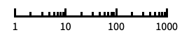
自動目盛ラベル付きの対数スケール "Log10" 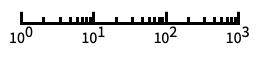
10のベキ乗に目盛が付いた,10を底とする対数スケール "SignedLog" 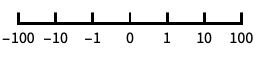
0と負の数を含む対数に似たスケール "Reverse" 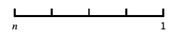
座標の向きを逆にする "Infinite" 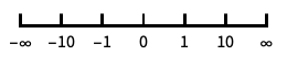
無限スケール - 一般に,x または y 軸と r 軸を同時にスケールすることはできない.
全オプションのリスト
例題
すべて開く すべて閉じる例 (3)
ListPolarPlot[Table[Sqrt[n], {n, 100}]]ListPolarPlot[Table[Sqrt[n], {n, 100}], Joined -> True]ListPolarPlot[Table[{n, Log[n]}, {n, 500}]]ListPolarPlot[{Range[100] / 4, Sqrt[Range[100]], Log[Range[100]]}, DataRange -> {0, 2Pi}, PlotLegends -> {"one", "two", "three"}]スコープ (29)
データ (9)
r の値からなる規則的なデータでは,θ のデータ範囲は等間隔で置かれる:
ListPolarPlot[Sqrt[Range[20]], Joined -> True]DataRangeを使い,θ のデータ範囲を明示的に与える:
ListPolarPlot[Sqrt[Range[20]], DataRange -> {0, 4Pi}, Joined -> True]ListPolarPlot[{Sqrt[Range[40]], Log[Range[40, 80]]}, Joined -> True]θ, r 値のペアからなる不規則なデータの場合,θ のデータ範囲はデータより推測される:
data = Table[{i, i + 1}, {i, 100}];ListPolarPlot[data, Joined -> True, Ticks -> None]data1 = Table[{i, i}, {i, 30}];
data2 = Table[{i + 1 / 3, i}, {i, 30}];
data3 = Table[{i + 2 / 3, i}, {i, 30}];ListPolarPlot[{data1, data2, data3}, Joined -> True]ListPolarPlot[{1, 2, 3, 1 + I, 4, 5, 6, None, 7, 8, 9, Missing["NotAvailable"], 10, 11, 12}, Joined -> True, Mesh -> All]ListPolarPlot[Sqrt[Sin[Range[0, 3Pi, 0.1]]], Joined -> True]MaxPlotPointsを使って使用する点の数を制限する:
Table[ListPolarPlot[Table[Sin[4i], {i, 0, 2Pi, 2Pi / 100}], MaxPlotPoints -> mp, Joined -> True], {mp, {Infinity, 50, 30}}]PlotRangeは自動的に選択される:
ListPolarPlot[Table[{θ, θ ^ (-1 / 2)}, {θ, 0.1, 25, 0.05}], Joined -> True]PlotRangeを使って関心領域に焦点を当てる:
{ListPolarPlot[Table[{θ, θ ^ (-1 / 2) + RandomReal[0.01]}, {θ, 1, 50, 0.02}], Joined -> True], ListPolarPlot[Table[{θ, θ ^ (-1 / 2) + RandomReal[0.01]}, {θ, 1, 50, 0.02}], Joined -> True, PlotRange -> 0.2]}TimeSeriesをプロットする:
r = Table[Mod[i, 3], {i, 0, 9, 1 / 2}];
angles = Range[0, π, π / (Length[r] - 1)];
ts = TimeSeries[r, {angles}]ListPolarPlot[ts, Joined -> True]表形式データ (1)
tabular = Tabular[IconizedObject[«spirals»], {"θ", "r", "s", "p"}]ListPolarPlot[tabular -> {"θ", "r"}, Joined -> True]角度に沿って等間隔に置かれた半径 r のリストをプロットする:
ListPolarPlot[tabular -> "θ", Joined -> True]ListPolarPlot[tabular -> {{"θ", "r"}, {"θ", "s"}}, Joined -> True]ラベル付けと凡例 (10)
ListPolarPlot[Sqrt[Range[13]] -> CharacterRange["a", "m"]]Calloutを使って点の集合にラベルを加える:
ListPolarPlot[Callout[Cos[ Range[0, 4Pi, 0.1]], "label"]]ListPolarPlot[Callout[Cos[Range[0, 4Pi, 0.1]], "label", {0.5, 0.5}]]ListPolarPlot[Callout[Sin[Range[0, 4Pi, 0.1]], "label", Scaled[0.15]]]Table[ListPolarPlot[Callout[Sin[Range[0, 4Pi, 0.1]], "label", pos], PlotLabel -> pos], {pos, {Top, Bottom}}]Table[ListPolarPlot[Callout[Sin[Range[0, 4Pi, 0.1]], "label", pos], PlotLabel -> pos], {pos, {Above, Below}}]PlotLabelsでデータにラベルを付ける:
ListPolarPlot[Sin[Range[0, 4Pi, 0.1]], PlotLabels -> "label"]ListPolarPlot[{Cos[Range[0, 2Pi, 0.1]], Sin[Range[0, 2Pi, 0.1]]}, PlotLabels -> {"cosine", "sine"}]ListPolarPlot[Callout[Sqrt[Range[100]], "label", Scaled[0.85]]]ListPolarPlot[Callout[Sqrt[Range[100]], "label", {Scaled[0.85], Below}]]ListPolarPlot[Callout[Sqrt[Range[100]], "label", {5, -4}]]ListPolarPlot[Range[100], Joined -> True, DataRange -> {1, 10}, ScalingFunctions -> {"Reverse", None}]ListPolarPlot[Range[100], Joined -> True, DataRange -> {1, 10}, ScalingFunctions -> {None, None, None, "Log"}]プレゼンテーション (9)
Joinedを使い,データ集合を線で繋ぐ:
ListPolarPlot[Range[10], Joined -> True, PlotStyle -> Orange]data = Table[Table[{x, f}, {x, 0, 2Pi, 0.05}], {f, {Sin[2x], Sin[4x]}}];ListPolarPlot[data, Joined -> True]data = Table[Table[{x, f}, {x, 0, 2Pi, 0.05}], {f, {Sin[2x], Sin[4x]}}];ListPolarPlot[data, PlotStyle -> {Dashed, Red}, Joined -> True]ListPolarPlot[Table[{θ, GoldenRatio ^ θ}, {θ, 0, 4Pi, 0.25}], Joined -> True, AxesLabel -> {r, r}, PlotLabel -> GoldenRatio ^ θ, PlotStyle -> Directive[PointSize[Medium], Purple], Mesh -> All]データにインタラクティブなTooltipを与える:
ListPolarPlot[Tooltip[Table[x, {x, 1, 25}]], PlotStyle -> Directive[PointSize[Medium], Orange]]data = Table[Tooltip[Table[{θ, f}, {θ, 0, 2Pi, 0.05}], TraditionalForm[f]], {f, {Sin[2θ], Sin[4θ]}}];ListPolarPlot[data, Joined -> True]ListPolarPlot[Table[p ^ n, {p, 1.1, 1.4, 0.1}, {n, 0, 5, 0.2}], PlotMarkers -> Automatic]ListPolarPlot[Table[Sin[p] ^ n, {p, 1.1, 1.4, 0.1}, {n, 0, 5, 0.2}], PlotMarkers -> Automatic, PlotLegends -> Range[1.1, 1.4, 0.1]]Legendedを使って追加的な凡例を加える:
{data1, data2, data3, data4} = Table[Sin[p] ^ n, {p, 1.1, 1.4, 0.1}, {n, 0, 5, 0.2}];ListPolarPlot[{data1, data2, data3, Legended[data4, HoldForm[Sin[1.4] ^ n]]}, Joined -> True, PlotLegends -> Range[1.1, 1.4, 0.1]]InterpolationOrderを使って繋いだデータを滑らかにする:
Table[ListPolarPlot[Range[10], Joined -> True, InterpolationOrder -> io, PlotStyle -> Dashed], {io, {0, 1, 2, 3}}]ListPolarPlot[Table[{n, Log[n]}, {n, 500}], PlotTheme -> "Marketing"]オプション (102)
ColorFunction (5)
ColorFunctionはJoinedされたデータ集合のみに適用される:
{ListPolarPlot[Sin[Range[0, 4Pi, 0.1]], ColorFunction -> "Rainbow"], ListPolarPlot[Sin[Range[0, 4Pi, 0.1]], ColorFunction -> "Rainbow", Joined -> True]}


Table[ListPolarPlot[Abs[Sin[Range[0, 4Pi, 0.1]]], Joined -> True, ColorFunction -> Function[{x, y, θ, r}, Evaluate[f]], PlotLabel -> f, PlotStyle -> Thick], {f, {Hue[x], Hue[y], Hue[θ], Hue[r]}}]ListPolarPlot[Sin[Range[0, 4Pi, 0.1]], Joined -> True, ColorFunction -> "DarkRainbow"]ColorFunctionは曲線の彩色に関してPlotStyleより優先順位が高い:
ListPolarPlot[Sin[Range[0, 4Pi, 0.1]], Joined -> True, ColorFunction -> "DarkRainbow", PlotStyle -> Directive[Red, Thick]]ColorFunctionを使うためにMeshShadingにAutomaticを使う:
ListPolarPlot[Sin[Range[0, 4Pi, 0.1]], Joined -> True, ColorFunction -> Function[{x, y, θ, r}, Hue[θ]], PlotStyle -> Directive[Red, Thick], Mesh -> 15, MeshShading -> {Automatic, StandardGray}, MeshStyle -> None]ColorFunctionScaling (3)
ColorFunctionScalingはJoinedされたデータ集合のみに適用される:
{ListPolarPlot[Range[10], ColorFunction -> "Rainbow", ColorFunctionScaling -> True], ListPolarPlot[Range[10], Joined -> True, ColorFunction -> "Rainbow", ColorFunctionScaling -> True]}ListPolarPlot[Sin[Range[0, 4Pi, 0.1]], Joined -> True, ColorFunction -> Function[{x, y, θ, r}, ColorData["RedBlueTones"][r]], PlotStyle -> Thick, ColorFunctionScaling -> True]ListPolarPlot[Sin[Range[0, 4Pi, 0.1]], Joined -> True, ColorFunction -> Function[{x, y, θ, r}, ColorData["RedBlueTones"][Abs[r]]], PlotStyle -> Thick, ColorFunctionScaling -> False]DataRange (4)
ListPolarPlot[Table[1, {i, 25}]]ListPolarPlot[Range[100], DataRange -> {0, 4Pi}]ListPolarPlot[{Sin[Range[0, 8Pi, 0.1]], Sin[Range[0, 4Pi, 0.1]]}, DataRange -> {0, 2Pi}, Joined -> True]ListPolarPlot[Table[{3t, 1}, {t, 0, 2Pi, 2Pi / 10}], Joined -> True]この場合,DataRangeを指定することは θ の値がデータの一部なので無意味である:
ListPolarPlot[Table[{3t, 1}, {t, 0, 2Pi, 2Pi / 10}], Joined -> True, DataRange -> {0, 1}]ImageSize (7)
Tiny,Small,Medium,Largeのような名前付きのサイズを使う:
{ListPolarPlot[Table[Sin[t], {t, 0, 4Pi, Pi / 50}], ImageSize -> Tiny], ListPolarPlot[Table[Sin[t], {t, 0, 4Pi, Pi / 50}], ImageSize -> Small]}{ListPolarPlot[Table[Sin[t], {t, 0, 4Pi, Pi / 50}], ImageSize -> 150], ListPolarPlot[Table[Sin[t], {t, 0, 4Pi, Pi / 50}], AspectRatio -> 1.5, ImageSize -> 150]}{ListPolarPlot[Table[Sin[t], {t, 0, 4Pi, Pi / 50}], ImageSize -> {Automatic, 150}], ListPolarPlot[Table[Sin[t], {t, 0, 4Pi, Pi / 50}], AspectRatio -> 2, ImageSize -> {Automatic, 150}]}{ListPolarPlot[Table[Sin[t], {t, 0, 4Pi, Pi / 50}], ImageSize -> UpTo[200]], ListPolarPlot[Table[Sin[t], {t, 0, 4Pi, Pi / 50}], AspectRatio -> 2, ImageSize -> UpTo[200]]}グラフィックスの幅と高さを指定し,必要であれば空間で充填する:
ListPolarPlot[Table[Sin[t], {t, 0, 4Pi, Pi / 50}], ImageSize -> {200, 300}, Background -> StandardYellow]AspectRatioFullと設定すると使用可能な空間が充填される:
ListPolarPlot[Table[Sin[t], {t, 0, 4Pi, Pi / 50}], AspectRatio -> Full, ImageSize -> {200, 300}, Background -> StandardYellow]{ListPolarPlot[Table[Sin[t], {t, 0, 4Pi, Pi / 50}], ImageSize -> {UpTo[150], UpTo[100]}], ListPolarPlot[Table[Sin[t], {t, 0, 4Pi, Pi / 50}], AspectRatio -> 2, ImageSize -> {UpTo[150], UpTo[100]}]}ImageSizeFullを使ってオブジェクトの使用可能な空間を塗り潰す:
Framed[Pane[ListPolarPlot[Table[Sin[t], {t, 0, 4Pi, Pi / 50}], ImageSize -> Full, Background -> StandardYellow], {200, 200}]]Framed[Pane[ListPolarPlot[Table[Sin[t], {t, 0, 4Pi, Pi / 50}], AspectRatio -> Full, ImageSize -> {Scaled[0.5], Scaled[0.5]}, Background -> StandardYellow], {200, 200}]]InterpolationOrder (5)
Joinedされる線を補間することができる:
ListPolarPlot[Range[10], Joined -> True, InterpolationOrder -> 2]ListPolarPlot[Range[10], Joined -> True, InterpolationOrder -> None, Mesh -> Full]ListPolarPlot[Range[10], Joined -> True, InterpolationOrder -> 0, Mesh -> Full]ListPolarPlot[{{1, 4, 2, 3, 10, 8, 2}}, Joined -> True, InterpolationOrder -> 3, Mesh -> Full]Table[ListPolarPlot[{{1, 4, 2, 3, 10, 8, 2}}, Joined -> True, InterpolationOrder -> i, Mesh -> Full, PlotLabel -> i], {i, 0, 5}]Joined (3)
ListPolarPlot[Sqrt[Range[20]], Joined -> True]ListPolarPlot[{Sqrt[Range[20]], Range[0, 10, 0.1]}, Joined -> {True, False}]ListPolarPlot[Range[20], Joined -> True, Mesh -> All]LabelingFunction (7)
ListPolarPlot[Table[x, {x, 1, 10}] -> {"a", "b", "c", "d", "e", "f", "g", "h", "i", "j"}]LabelingFunction->Noneを使ってラベルを付けないようにする:
ListPolarPlot[Table[x, {x, 1, 10}] -> {"a", "b", "c", "d", "e", "f", "g", "h", "i", "j"}, LabelingFunction -> None]ListPolarPlot[Table[x, {x, 1, 10}] -> {"a", "b", "c", "d", "e", "f", "g", "h", "i", "j"}, LabelingFunction -> Above]ListPolarPlot[Table[x, {x, 1, 10}] -> {"a", "b", "c", "d", "e", "f", "g", "h", "i", "j"}, LabelingFunction -> Tooltip]Calloutを使って点にラベルを付ける:
ListPolarPlot[Table[x, {x, 1, 10}] -> {"a", "b", "c", "d", "e", "f", "g", "h", "i", "j"}, LabelingFunction -> Callout[Automatic, Appearance -> "Line"]]ListPolarPlot[Table[x, {x, 1, 10}] -> {"a", "b", "c", "d", "e", "f", "g", "h", "i", "j"}, LabelingFunction -> (Round[#1, 0.1]&)]ListPolarPlot[Table[x, {x, 1, 10}] -> {"a", "b", "c", "d", "e", "f", "g", "h", "i", "j"}, LabelingFunction -> (#2[[2]]&)]全体的なラベルをPlotLabelsで指定し,個々のラベルをTooltipで置く:
ListPolarPlot[Table[x, {x, 1, 10}] -> {"a", "b", "c", "d", "e", "f", "g", "h", "i", "j"}, PlotLabels -> {"label"}, Joined -> True, PlotMarkers -> Automatic, LabelingFunction -> (Placed[#3, Tooltip]&)]LabelingSize (2)
ListPolarPlot[Callout[Cos[Sin[2Pi Subdivide[100]]], "ListPolarPlot", {0.5, -0.5}]]ListPolarPlot[Callout[Cos[Sin[Range[0, 2Pi, 0.1]]], "ListPolarPlot", {0.5, -0.5}], LabelingSize -> 30]ListPolarPlot[Callout[Cos[Sin[Range[0, 2Pi, 0.1]]], [image], {0.5, -0.5}]]ListPolarPlot[Callout[Cos[Sin[Range[0, 2Pi, 0.1]]], [image], {0.5, -0.5}], LabelingSize -> 60]LabelingTarget (6)
ListPolarPlot[IconizedObject[«data»]]ListPolarPlot[IconizedObject[«data»], LabelingTarget -> All]ListPolarPlot[IconizedObject[«data»], LabelingTarget -> "Dense"]ListPolarPlot[IconizedObject[«data»], LabelingTarget -> 0.5]ListPolarPlot[IconizedObject[«data»], LabelingTarget -> <|"AllowedLabelingPositions" -> "Sides"|>]ListPolarPlot[IconizedObject[«data»], LabelingTarget -> <|"AllowedLabelingPositions" -> "Corners"|>]ListPolarPlot[IconizedObject[«data»], LabelingTarget -> <|"AllowedLabelingPositions" -> {"Top", "Right"}, "AllowedOverlaps" -> {"Lines"}|>]ListPolarPlot[IconizedObject[«data»], LabelingTarget -> <|"AllowLabelClipping" -> True|>]MaxPlotPoints (2)
ListPolarPlot[Table[Sin[t], {t, 0, 4Pi, Pi / 100}], Joined -> True]Table[ListPolarPlot[Table[Sin[t], {t, 0, 4Pi, Pi / 100}], MaxPlotPoints -> mp, Joined -> True], {mp, {Infinity, 50, 30}}]

ListPolarPlot[Sin[Range[10^6]2.Pi / 10^5] + RandomReal[0.3, 10^6], MaxPlotPoints -> 10^3, Joined -> True]Mesh (6)
{ListPolarPlot[Table[Sin[t], {t, 0, 4Pi, 0.2}], Mesh -> 31], ListPolarPlot[Table[Sin[t], {t, 0, 4Pi, 0.2}], Mesh -> 31, Joined -> True]}{ListPolarPlot[Table[Sin[t], {t, 0, 4Pi, 0.2}], Mesh -> Full, Joined -> True], ListPolarPlot[Table[Sin[t], {t, 0, 4Pi, 0.2}], Mesh -> All, Joined -> True]}{ListPolarPlot[Table[Sin[t], {t, 0, 4Pi, 0.2}], Mesh -> Full, InterpolationOrder -> 3, Joined -> True], ListPolarPlot[Table[Sin[t], {t, 0, 4Pi, 0.2}], Mesh -> All, InterpolationOrder -> 3, Joined -> True]}ListPolarPlot[Table[Sin[t], {t, 0, 4Pi, 0.2}], Mesh -> 20, Joined -> True]ListPolarPlot[Table[Sin[t], {t, 0, 4Pi, 0.2}], Mesh -> {Range[0, 2Pi, Pi / 8]}, MeshStyle -> PointSize[Medium], Joined -> True]ListPolarPlot[Table[Sin[t], {t, 0, 4Pi, 0.2}], Mesh -> {Table[{x, Directive[Hue[x / (2Pi)], PointSize[Medium]]}, {x, 0, 2Pi, Pi / 8}]}, Joined -> True]MeshFunctions (3)
MeshFunctionsはJoinedのデータ集合のみに適用される:
{ListPolarPlot[Table[Sin[t], {t, 0, 4Pi, 0.2}], Mesh -> 10, MeshFunctions -> {#1&}], ListPolarPlot[Table[Sin[t], {t, 0, 4Pi, 0.2}], Mesh -> 10, MeshFunctions -> {#1&}, Joined -> True]} 方向,
 方向,
 方向,
 方向に等間隔で置かれたメッシュを使う:
Table[ListPolarPlot[Table[Sin[t], {t, 0, 4Pi, 0.2}], MeshFunctions -> {Function[{x, y, θ, r}, Evaluate[f]]}, Mesh -> 16, PlotLabel -> f, Joined -> True], {f, {x, y, θ, r}}] 方向に赤いメッシュを5レベル,
 方向に青いメッシュを10レベル使う:
ListPolarPlot[Table[Sin[t], {t, 0, 4Pi, 0.2}], Mesh -> {5, 10}, MeshFunctions -> {#1&, #2&}, MeshStyle -> {Directive[PointSize[Medium], Red], Blue}, Joined -> True]MeshShading (7)
MeshShadingはJoinedのデータ集合のみに適用される:
{ListPolarPlot[Table[Sin[t], {t, 0, 4Pi, 0.2}], Mesh -> 10, MeshShading -> {Red, Blue}], ListPolarPlot[Table[Sin[t], {t, 0, 4Pi, 0.2}], Mesh -> 10, MeshShading -> {Red, Blue}, Joined -> True]}ListPolarPlot[Table[Sin[t], {t, 0, 4Pi, 0.2}], Mesh -> 10, MeshShading -> {Red, Blue}, Joined -> True]Noneを使って線分を除去する:
ListPolarPlot[Table[Sin[t], {t, 0, 4Pi, 0.2}], Mesh -> 10, MeshShading -> {Red, None}, Joined -> True]MeshShadingはPlotStyleとともに使うことができる:
ListPolarPlot[Table[Sin[t], {t, 0, 4Pi, 0.2}], Mesh -> 10, PlotStyle -> Thick, MeshShading -> {Red, Blue}, Joined -> True]MeshShadingは曲線のスタイル付けに関しPlotStyleより優先順位が高い:
ListPolarPlot[Table[Sin[t], {t, 0, 4Pi, 0.2}], Mesh -> 10, PlotStyle -> Green, MeshShading -> {Red, Blue}, Joined -> True]MeshShadingをAutomaticにし,線分にPlotStyleを使う:
ListPolarPlot[Table[Sin[t], {t, 0, 4Pi, 0.2}], Mesh -> 10, PlotStyle -> Directive[Thick, Yellow], MeshShading -> {Red, Automatic}, Joined -> True]MeshShadingはColorFunctionとともに使うことができ,優先度が高い:
ListPolarPlot[Table[Sin[t], {t, 0, 4Pi, 0.2}], Mesh -> 30, PlotStyle -> Thick, MeshShading -> {StandardGray, Automatic},
	ColorFunction -> Function[{x, y, θ, r}, Hue[θ]], Joined -> True]
MeshStyle (5)
MeshStyleはJoinedのデータ集合のみに適用される:
{ListPolarPlot[Table[Sin[t], {t, 0, 4Pi, 0.2}], Mesh -> 10, MeshStyle -> Red], ListPolarPlot[Table[Sin[t], {t, 0, 4Pi, 0.2}], Mesh -> 10, MeshStyle -> Red, Joined -> True]}ListPolarPlot[Table[Sin[t], {t, 0, 4Pi, 0.2}], Mesh -> 10, MeshStyle -> Automatic, Joined -> True]
ListPolarPlot[Table[Sin[t], {t, 0, 4Pi, 0.2}], Mesh -> 10, MeshStyle -> Red, Joined -> True]

ListPolarPlot[Table[Sin[t], {t, 0, 4Pi, 0.2}], Mesh -> 10, MeshStyle -> {Red, Blue}, MeshFunctions -> {#1&, #2&}, Joined -> True]ListPolarPlot[Table[Sin[t], {t, 0, 4Pi, 0.2}], Mesh -> 15, MeshStyle -> Directive[PointSize[Large], Red], Joined -> True]PlotLabels (5)
ListPolarPlot[{Sin[Range[0, 2Pi, 0.1]], Cos[Range[0, 2Pi, 0.1]]}, PlotLabels -> Callout[{"sin", "cos"}, After]]ListPolarPlot[{Sin[Range[0, 2Pi, 0.1]], Cos[Range[0, 2Pi, 0.1]]}, PlotLabels -> Callout[{"label1", "label2"}, Above]]ListPolarPlot[{Sin[Range[0, 2Pi, 0.1]], Cos[Range[0, 2Pi, 0.1]]}, PlotLabels -> {Callout["label1", Above], Callout["label2", After]}]ListPolarPlot[{Sin[Range[0, 2Pi, 0.1]], Cos[Range[0, 2Pi, 0.1]]}, PlotLabels -> {Callout["label1", {Scaled[0.7], Above}], Callout["label2", {Scaled[0.4], Below}]}]ListPolarPlot[{Sin[Range[0, 2Pi, 0.1]], Cos[Range[0, 2Pi, 0.1]]}, PlotLabels -> {Callout["label1", Before], Callout["label2", After]}]Noneを使ってラベルを加えないようにする:
ListPolarPlot[{Sin[Range[0, 2Pi, 0.1]], Cos[Range[0, 2Pi, 0.1]]}, PlotLabels -> {"label1", None}]PlotLegends (7)
ListPolarPlot[Sin[Range[0, 4Pi, 0.1]]]ListPolarPlot[{Sin[Range[0, 4Pi, 0.1]], Cos[Range[0, 4Pi, 0.1]]}, PlotStyle -> {Red, Blue}, PlotLegends -> {"sine", "cose"}]ListPolarPlot[{Sin[Range[0, 8Pi, 0.1]], Sin[Range[0, 4Pi, 0.1]]}, PlotLegends -> Automatic]ListPolarPlot[{Sin[Range[0, 8Pi, 0.1]], Sin[Range[0, 4Pi, 0.1]]}, PlotStyle -> {Directive[AbsolutePointSize[5], Red], Blue}, PlotLegends -> Automatic]Placedを使って凡例の置き方を指定する:
Table[ListPolarPlot[{Sin[Range[0, 8Pi, 0.1]], Sin[Range[0, 4Pi, 0.1]]}, PlotLegends -> Placed[Automatic, pl], PlotLabel -> pl], {pl, {After, Before}}]ListPolarPlot[{Range[40], Range[40] ^ 1.2}, PlotLegends -> Placed[PointLegend[Automatic, LegendLayout -> "Row"], {0.75, 0.85}]]Table[ListPolarPlot[{Sin[Range[0, 8Pi, 0.1]], Sin[Range[0, 4Pi, 0.1]]}, PlotLegends -> Placed[Automatic, pl]], {pl, {After, Above}}]PointLegendを使って凡例の外観を変える:
ListPolarPlot[{Sin[Range[0, 8Pi, 0.1]], Sin[Range[0, 4Pi, 0.1]]}, PlotLegends -> PointLegend[{8, 4}, LegendFunction -> Panel, LegendLayout -> "Row"]]PlotMarkers (8)
ListPolarPlotは,一般に,データを区別するために異なる色を使う:
ListPolarPlot[Table[p ^ n, {p, 1.1, 1.4, 0.1}, {n, 0, 5, 0.2}], PlotMarkers -> None]ListPolarPlot[Table[p ^ n, {p, 1.1, 1.4, 0.1}, {n, 0, 5, 0.2}], PlotMarkers -> Automatic]ListPolarPlot[Table[p ^ n, {p, 1.1, 1.4, 0.1}, {n, 0, 5, 0.2}], PlotMarkers -> Automatic, PlotStyle -> StandardBlue]Table[ListPolarPlot[Table[p ^ n, {p, 1.1, 1.4, 0.1}, {n, 0, 5, 0.2}], PlotMarkers -> {Automatic, s}], {s, {Small, Medium}}]ListPolarPlot[Table[p ^ n, {p, 1.1, 1.4, 0.1}, {n, 0, 5, 0.2}], PlotMarkers -> {Automatic, Large}]ListPolarPlot[Table[p ^ n, {p, 1.1, 1.4, 0.1}, {n, 0, 5, 0.2}], PlotMarkers -> {"1", "2", "3", "4"}]{m1, m2, m3, m4} = Graphics /@ {Circle[{0, 0}, 1], Disk[{0, 0}, 1], Line[{{-0.5, -0.5}, {0.5, -0.5}, {0.5, 0.5}, {-0.5, 0.5}, {-0.5, -0.5}}], Polygon[{{-0.5, -0.5}, {0.5, -0.5}, {0.5, 0.5}, {-0.5, 0.5}}]}ListPolarPlot[Table[p ^ n, {p, 1.1, 1.4, 0.1}, {n, 0, 5, 0.2}], PlotMarkers -> Table[{s, 0.05}, {s, {m1, m2, m3, m4}}]]ListPolarPlot[Table[p ^ n, {p, 1.1, 1.4, 0.1}, {n, 0, 5, 0.2}], PlotMarkers -> "●"]Table[ListPolarPlot[Table[p ^ n, {p, 1.1, 1.4, 0.1}, {n, 0, 5, 0.2}], PlotMarkers -> {"●", s}], {s, {4, 8, 12}}]PlotRange (2)
PlotRangeは自動的に計算される:
ListPolarPlot[{1, 2, 3, 4, 50, 6, 7, 8, 9, 10, 11, 12}, Joined -> True]ListPolarPlot[{1, 2, 3, 4, 50, 6, 7, 8, 9, 10, 11, 12}, Joined -> True, PlotRange -> All]PlotStyle (7)
Table[ListPolarPlot[Table[k / 10, {k, 0, 2Pi, 0.2}], PlotStyle -> ps], {ps, {Red, PointSize[Large], Darker[Green], Directive[Red, PointSize[Large]]}}]Table[ListPolarPlot[Table[k / 10, {k, 0, 2Pi, 0.2}], PlotStyle -> ps, Joined -> True], {ps, {Red, Thick, Darker[Green], Directive[Red, Dashed]}}]ListPolarPlot[Table[k, {k, 1, 3}, {50}]]ListPolarPlot[Table[k, {k, 1, 3}, {50}], PlotStyle -> {Red, Green, Blue}]PlotStyleは線と点の両方に適用される:
ListPolarPlot[Table[k, {k, 1, 2}, {50}], Joined -> {True, False}, PlotStyle -> Red]ListPolarPlot[Table[k, {k, 1, 2}, {50}], Joined -> {True, False}, PlotStyle -> {Thick, PointSize[Large]}]PlotStyleはColorFunctionと組み合せることができる:
ListPolarPlot[Table[Sin[4x], {x, 0, 2Pi, 0.05}], Joined -> True, PlotStyle -> Thick, ColorFunction -> Function[{x, y, θ, r}, Hue[θ]]]PlotStyleはMeshShadingは組み合せて使用できるが,優先度は低い:
ListPolarPlot[Table[Sin[4x], {x, 0, 2Pi, 0.05}], Joined -> True, PlotStyle -> Directive[Opacity[0.5], Thick], Mesh -> 10, MeshFunctions -> {#1&}, MeshShading -> {Red, Blue}]MeshStyleはデフォルトでPlotStyleと同じスタイルに設定されている:
ListPolarPlot[Table[Sin[4x], {x, 0, 2Pi, 0.05}], PlotStyle -> Red, Mesh -> All, Joined -> True]PlotTheme (1)
ListPolarPlot[Sin[Range[0, 4Pi, 0.1]], Joined -> True, PlotTheme -> "Scientific"]ListPolarPlot[Sin[Range[0, 4Pi, 0.1]], Joined -> True, PlotTheme -> {"Scientific", "Grid"}]ListPolarPlot[Sin[Range[0, 4Pi, 0.1]], Joined -> True, PlotTheme -> {"Scientific", "Grid"}, ColorFunction -> "DarkRainbow"]PolarAxes (1)
ListPolarPlot[Table[{t, 2Sin[2t]}, {t, 0, 2π, π / 100}], PlotRangePadding -> 2, PolarAxes -> True]ListPolarPlot[Table[{t, 2Sin[2t]}, {t, 0, 2π, π / 100}], PlotRangePadding -> 2, PolarAxes -> True, PolarGridLines -> True]ListPolarPlot[Table[{t, 2Sin[2t]}, {t, 0, 2π, π / 100}], PlotRangePadding -> 2, PolarAxes -> {True, False}, PolarGridLines -> True]PolarAxesOrigin (1)


ListPolarPlot[Table[{{θ, 2Sin[2θ]}, {θ, Cos[2θ]}}, {θ, 0, 2π, 0.01}], PlotRangePadding -> 4, PolarAxes -> True, PolarAxesOrigin -> {0, 3}]ListPolarPlot[Table[{{θ, 2Sin[2θ]}, {θ, Cos[2θ]}}, {θ, 0, 2π, 0.01}], PlotRangePadding -> 1.5, PolarAxes -> True, PolarAxesOrigin -> {{Bottom, Right}, Automatic}, PolarTicks -> {None, Automatic}]PolarGridLines (1)
ListPolarPlot[Table[{θ, 3Cos[3θ]}, {θ, 0, 2Pi, 0.1}], PlotRangePadding -> 2.5, PolarAxes -> True, PolarGridLines -> Automatic]ListPolarPlot[Table[{θ, 3Cos[3θ]}, {θ, 0, 2Pi, 0.1}], PlotRangePadding -> 1.5, PolarAxes -> True, PolarGridLines -> {{0, (2π/3), (4π/3)}, Automatic}, PolarTicks -> {{0, (2π/3), (4π/3)}, Automatic}]ListPolarPlot[Table[{θ, 3Cos[3θ]}, {θ, 0, 2Pi, 0.1}], GridLinesStyle -> Orange, PlotRangePadding -> 1.5, PolarAxes -> True, PolarGridLines -> {{0, (2π/3), (4π/3)}, Automatic}, PolarTicks -> {{0, (2π/3), (4π/3)}, Automatic}]PolarTicks (1)
ListPolarPlot[Table[{θ, 1 - 2Sin[4θ]}, {θ, 0, 2Pi, 0.02}], PlotRangePadding -> 2.5, PolarAxes -> True, PolarTicks -> Automatic]角度が から
 までではなく
 から
 までになるように目盛ラベルのいくつかを変える:
ListPolarPlot[Table[{θ, 1 - 2Sin[4θ]}, {θ, 0, 2Pi, 0.02}], PlotRangePadding -> 2.5, PolarAxes -> True, PolarTicks -> {{0, (π/4), (π/2), (3 π/4), π, {(5 π/4), -(3π/4)}, {(3 π/2), -(π/2)}, {(7 π/4), -(π/4)}}, Automatic}]ListPolarPlot[Table[{θ, 1 - 2Sin[4θ]}, {θ, 0, 2Pi, 0.02}], PlotRangePadding -> 1.5, PolarAxes -> True, PolarTicks -> {"Degrees", Range[0, 3]}]ScalingFunctions (3)
デフォルトで,ListPolarPlotは両軸に自然スケールを使う:
ListPolarPlot[IconizedObject[«spiral»], Joined -> True]ScalingFunctionsを使って y 方向の座標方向を逆にする:
ListPolarPlot[IconizedObject[«spiral»], Joined -> True, ScalingFunctions -> {None, "Reverse", None, None}]ListPolarPlot[IconizedObject[«spiral»], Joined -> True, ScalingFunctions -> {None, None, None, "Log"}]特性と関係 (13)
ListPolarPlotはListPlotの特殊ケースである:
{ListPolarPlot[Table[k, {k, 0, 9}], Joined -> True],
ListPlot[Table[{k Cos[2Pi k / 10], k Sin[2Pi k / 10]}, {k, 0, 9}], Joined -> True, AspectRatio -> Automatic]}関数にPolarPlotを使う:
{PolarPlot[Sin[4x], {x, 0, 2Pi}], ListPolarPlot[Table[{x, Sin[4x]}, {x, 0, 2Pi, 0.05}], Joined -> True]}直交座標でのプロットにListPlotとListLinePlotを使う:
ListPlot[Table[{x, Sqrt[x]}, {x, 0, 2Pi, 0.1}]]対数プロットにListLogPlot, ListLogLogPlot, ListLogLinearPlotを使う:
ListLogPlot[Table[Binomial[25, k], {k, 0, 25}], Joined -> True]データを時間に対して示すのにDateListPlotを使う:
DateListPlot[{5, 11, 13, 24, 28, 31, 34, 39, 42, 47, 51, 66}, {2006, 1}, PlotStyle -> PointSize[Medium]]三次元の点を示すのにListPointPlot3Dを使う:
ListPointPlot3D[Table[Sin[j ^ 2 + i], {i, 0, Pi, 0.1}, {j, 0, Pi, 0.1}]]データから曲面プロットを作るのにListPlot3Dを使う:
ListPlot3D[Table[Sin[j ^ 2 + i], {i, 0, Pi, 0.1}, {j, 0, Pi, 0.1}]]連続データから等高線プロットを作るのにListContourPlotを使う:
ListContourPlot[Table[Sin[j ^ 2 + i], {i, 0, Pi, 0.1}, {j, 0, Pi, 0.1}]]連続データから密度プロットを作るのにListDensityPlotを使う:
ListDensityPlot[Table[Sin[j ^ 2 + i], {i, 0, Pi, 0.1}, {j, 0, Pi, 0.1}]]離散値の配列にArrayPlotとMatrixPlotを使う:
ArrayPlot[Table[GCD[i, j], {i, 1, 20}, {j, 1, 20}]]円柱座標,球座標のプロットにRevolutionPlot3DとSphericalPlot3D を使う:
RevolutionPlot3D[-(ϕ + Sin[r]), {r, 0, 4Pi}, {ϕ, 0, 2Pi}]SphericalPlot3D[1 + 1 / 5Sin[3v], {u, 0, Pi}, {v, 0, 2Pi}]パラメトリック曲線にParametricPlotを使う:
{ParametricPlot[{Cos[θ], Sin[θ]}, {θ, 0, 2Pi}], ListLinePlot[Table[{Cos[θ], Sin[θ]}, {θ, 0, 2Pi, 0.1}], AspectRatio -> 1]}RadialAxisPlotは,円の周りに  次元の点座標を表示する:
{ListPolarPlot[Range[7], Joined -> True], RadialAxisPlot[Range[7]]}おもしろい例題 (1)
テキスト
Wolfram Research (2007), ListPolarPlot, Wolfram言語関数, https://reference.wolfram.com/language/ref/ListPolarPlot.html (2025年に更新).
CMS
Wolfram Language. 2007. "ListPolarPlot." Wolfram Language & System Documentation Center. Wolfram Research. Last Modified 2025. https://reference.wolfram.com/language/ref/ListPolarPlot.html.
APA
Wolfram Language. (2007). ListPolarPlot. Wolfram Language & System Documentation Center. Retrieved from https://reference.wolfram.com/language/ref/ListPolarPlot.html