



ListContourPlot
ListContourPlot[{{f11,…,f1n},…,{fm1,…,fmn}}]
値 fijの配列から等高線プロットを作成する.
ListContourPlot[{{x1,y1,f1},…,{xk,yk,fk}}]
点{xi,yi}で指定された値 fiから等高線プロットを生成する.
詳細とオプション
- ListContourPlotは,等値線,等値曲線,レベル集合,あるいはサブレベル集合プロットとしても知られている.
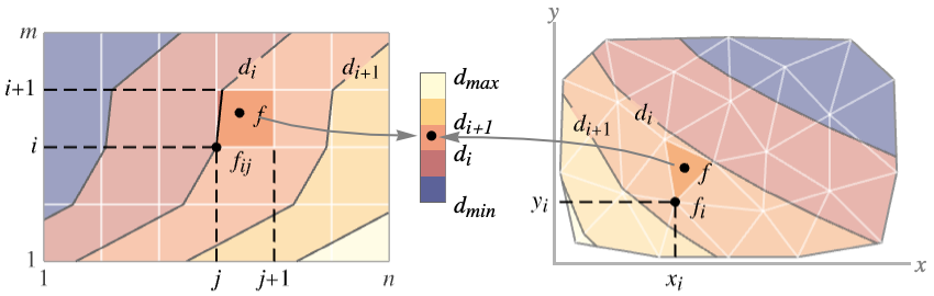
- 規則的なデータ{{f11,…,f1n},…,{fm1,…,fmn}}は関数 f[x,y]としてプロットされる.ただし,f[j,i]は点{x,y}で値 fijを持つ.
- 不規則データ{{x1,y1,f1},…,{xk,yk,fk}}は関数 f[x,y]としてプロットされる.ただし f[xi,yi]は点{x,y}で値 fiを持つ.
- ListContourPlotは f[x,y]が一定の値 d1, d2等を持つレベル集合に対応する等高曲線を構築する.デフォルトで,曲線間の領域は値が diから di+1までの領域が識別しやすくなるように陰影付される.
- この関数は領域
 を可視化する.ただし,f は上記の関数で領域
 は規則的なデータについてはデカルト積
 で不規則データについては{{x1,y1},…,{xn,yn}}の凸包である.
- 値 fijについての
 の位置は,規則的なデータ{{f11,…,f1n},…,{fm1,…,fmn}}の場合は
 であるとみなされる.オプションDataRangeを使ってこれを無効にする.
- デフォルトで,カラースケールが生成する出力では大きい値が明るい色で表示される.
- ListContourPlotは値の線形補間を行って滑らかな等高線を与える.
- データ値 xi,yi,ziは次の形式で与えられる.
-
xi 実数値の数 Quantity[xi,unit] 単位付きの数量 - ListContourPlot[data]は data について次の形と解釈を使うことができる.
-
{<xkeyx1,ykeyy1,fkeyf1>,…,<xkeyxn,ykeyyn,fkeyfn>} 不規則な3つ一組  ,{xi,yi,fi}
{{x1,y1},…,{xn,yn}}{f1,…,fn} 不規則な3つ一組  ,{xi,yi,fi}
Dataset 通常の配列としての値 NumericArray 通常の配列としての値 QuantityArray 大きさ SparseArray 通常の配列としての値 - ListContourPlot[Tabular[…]cspec]は,列指定 cspec を使って表形式オブジェクトから値を抽出し,
- 次は,表形式データのプロットに使用可能な列指定 cspec の形式である.
-
{colx,coly,colz} 列 z と列 x および列 y {{colx1,coly1,colz1},{colx2,coly2,colz2},…} 列 z1と列 x1および列 y1,列 z2と列 x2および列 y2等 - ListContourPlotはGraphicsのオプションと同じものに次の追加・訂正を加えたオプションを使う. [全オプションのリスト]
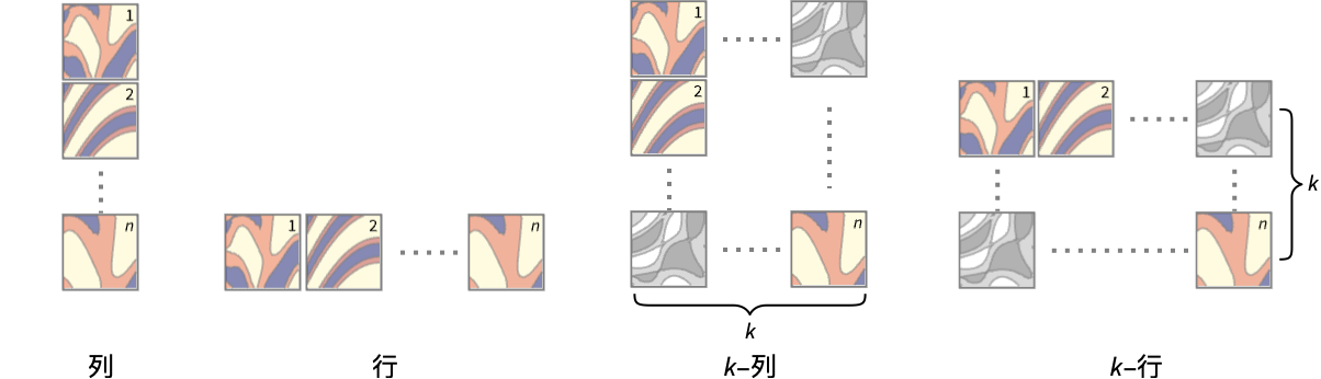
- 次は,複数のプロットパネルのそれぞれに単一の等高線を表示するPlotLayoutの可能な設定である.
-
"Column" パネルの列に別々の等高線を使う "Row" パネルの行に別々の等高線を使う {"Column",k},{"Row",k} k 列(または行)を使う {"Column",UpTo[k]},{"Row",UpTo[k]} 最大で k 列(または行)を使う - DataRangeは,配列{{f11,…,f1n},…,{fm1,…,fmn}}中の値 fijについて{x,y}の位置を決定する.次は,使用可能な設定である.
-
Automatic,All x は1から n まで,y は1から m まで一様 {{xmin,xmax},{ymin,ymax}} x は xminから xmaxまで,y は yminから ymaxまで一様 - ListContourPlot[{{a11,a12,a13},…}]の場合は規則的なデータと不規則データの両方に解釈できる.DataRange->Automaticとすると不規則な{{x1,y1,f1},{x2,y2,f2},…}と解釈され,DataRangeAllとすると規則的な{{f11,…,f1n},…,{fm1,…,fmn}}と解釈される.
- 等高線レベル間の領域にどのように色付けするかの決定する際,ListContourPlotはContourShading,ColorFunctionの順で,それぞれの明示的な設定を探す.
- ListContourPlotはSparseArrayオブジェクトと使うことができる.
- MeshFunctions,RegionFunctionの関数に渡される引数は x,y,f である.
- ColorFunctionにはデフォルトで,連続する等高線レベルの各ペアにつき,f のスケールされた値の平均によって与えられる1つの引数が与えられている.
- PlotLegendsのよく使われる設定値
-
None 凡例は置かない Automatic 凡例を自動的に決定する Placed[lspec,…] 凡例の置き方を指定する - ScalingFunctionsの可能な設定値
-
sf f 値をスケールする {sx,sy} x 軸と y 軸をスケールする {sx,sy,sf} x 軸,y 軸,f 値をスケールする - 各スケーリング関数 siは,文字列"scale"または{g,g-1}である.ただし,g-1は g の逆数である.
- ListContourPlotはGraphics[GraphicsComplex[data]]を返す.
全オプションのリスト
例題
すべて開く すべて閉じる例 (4)
ListContourPlot[Table[Sin[i + j ^ 2], {i, 0, 3, 0.1}, {j, 0, 3, 0.1}]]


data = Table[{x = RandomReal[{-2, 2}], y = RandomReal[{-2, 2}], Sin[x y]}, {1000}];ListContourPlot[data]ListContourPlot[RandomReal[1, {10, 10}], InterpolationOrder -> 3, PlotLegends -> Automatic]複数パネルのレイアウトを使って複数のデータ集合を同時に表示する:
ListContourPlot[{IconizedObject[«Subscript[data, 1]»], IconizedObject[«Subscript[data, 2]»]}, PlotLayout -> "Row"]スコープ (17)
データ (8)
 値からなる規則的なデータについて,
 と
 のデータ範囲は整数値であるとされる:
ListContourPlot[Table[Sin[x y], {x, 0, 3, 0.1}, {y, 0, 3, 0.1}], Mesh -> All]DataRangeを使って  と
 の明示的なデータ範囲を与える:
ListContourPlot[Table[Sin[x y], {x, 0, 3, 0.1}, {y, 0, 3, 0.1}], DataRange -> {{0, 3}, {0, 3}}] ,
 ,
 の3つ一組からなっている不規則データの場合,
 と
 のデータ範囲はデータから推測される:
data = Table[{x = RandomReal[{-1, 1}], y = RandomReal[{-1, 1}], x ^ 2 - y ^ 2}, {500}];ListContourPlot[data, Mesh -> All]ListContourPlot[ReplacePart[Partition[Range[100], 10], {{3, 3} -> None, {5, 7} -> I, {8, 4} -> Missing["NotAvailable"]}]]ListContourPlot[Table[{x = RandomReal[{-1, 1}], y = RandomReal[{-1, 1}], Sqrt[1 - x ^ 2 - y ^ 2]}, {1000}]]MaxPlotPointsを使って使用する点の数を制限する:
Table[ListContourPlot[Table[Sin[x y], {x, 0, 3, 0.075}, {y, 0, 3, 0.075}], MaxPlotPoints -> mp, Mesh -> All], {mp, {Infinity, 20, 10}}]PlotRangeは自動的に選択される:
ListContourPlot[Table[1 / (x ^ 2 + y ^ 2), {x, -2, 2, 4 / 51}, {y, -2, 2, 4 / 51}]]PlotRangeを使って関心領域に焦点を当てる:
{ListContourPlot[Table[x ^ 4 + y ^ 4 - x ^ 2 - y ^ 2 + 1, {x, -2, 2, 0.1}, {y, -2, 2, 0.1}]], ListContourPlot[Table[x ^ 4 + y ^ 4 - x ^ 2 - y ^ 2 + 1, {x, -2, 2, 0.1}, {y, -2, 2, 0.1}], PlotRange -> {0, 2}, ClippingStyle -> None]}RegionFunctionを使って不等式で与えられる範囲に密度プロットを限る:
data = Flatten[Table[{x, y, Sin[x ^ 2 + y ^ 2] / (x ^ 2 + y ^ 2)}, {x, -4, 4, 0.2}, {y, -4, 4, 0.2}], 1];//QuietListContourPlot[data, PlotRange -> All, RegionFunction -> Function[{x, y, z}, Norm[{x, y}] < 4]]表形式データ (1)
tabular = Tabular[Association["RawSchema" -> Association["ColumnProperties" ->
     Association["x" -> Association["ElementType" -> "Real64"],
      "y" -> Association["ElementType" -> "Real64"], "f" -> Association["ElementType" -> "Real64"],
      "g" -> Association["ElementType" -> "Real64"]], "KeyColumns" -> None,
    "Backend" -> "WolframKernel"], "BackendData" ->
   Association["ColumnData" -> DataStructure["ColumnTable",
      {{TabularColumn[Association["Data" -> {{-0.33582559210197255, 0.8803676729681109,
             -0.003450317591317193, -0.5776054861233806, -0.18944540146303104, 0.08137938087842855,
             0.7104751091887305, -0.7249989427695543, 0.7189171513953225, 0.07484856016827364,
             0.08394237912410371, -0.8397091750258563, -0.34613065738227494, 0.3153135739547788,
             0.1915099877033827, 0.6156751086440714, -0.6764522289849321, 0.42594752908865297,
             0.5452064158161848, -0.20490357958422162, 0.2656442175819875, 0.5930624991868867,
             -0.7653974593098988, -0.405399907196919, 0.4261842168600495, 0.007537997753683873,
             0.02320951605378001, 0.029467822857674145, -0.7726538362038052, -0.8906519148256042,
             -0.38273234260173566, -0.04463951504268252, -0.16350850917765758, 0.4690419314081237,
             -0.07389578232631427, -0.17270808669527418, -0.5037831593577057, -0.03935310416421582,
             0.15289554619000345, 0.4761074052545588, 0.01960730503071178, 0.346592918693779,
             -0.47057706227574775, -0.35440713666529167, -0.34731051462701956, -0.0457101610377397,
             0.04848867532803812, 0.04010379877047812, 0.36938420883956324, -0.10815861126341457,
             0.6830059609993497, -0.03055755892317922, 0.052870816573050865, 0.179789625890681,
             0.023635433559453523, -0.030528341731038623, -0.21544153070879574, 0.5826821668876411,
             -0.20600453971631344, -0.42604275708726047, -0.3929283758555415, -0.5043728799993309,
             0.04899025018573085, -0.6259318276915798, -0.7385675893002966, 0.02511690116030315,
             -0.4164641437703871, -0.44641422111020956, 0.05742014701654436, 0.18026818253918503,
             -0.25393260418265173, 0.6021117017355871, 0.37177688919047097, 0.11360855924293391,
             -0.25955329915886216, 0.5489751164992835, 0.23958190188503348, 0.39276345483198566,
             0.3478442618183317, -0.3456381030733422, 0.4225740854243536, 0.050722540211116975,
             -0.4339376582341843, -0.8928688667944833, 0.2875870676301678, 0.04838535997016681,
             0.17191625353893386, -0.040332095223106545, 0.2979213513808396, -0.25100379031925163,
             0.018748029889601718, 0.3372233005229358, 0.5402016231417128, 0.05153948798389716,
             0.06657679195492089, 0.507705731340098, 0.23183070367402803, 0.17700860995773013,
             -0.46345961004467046, -0.6014722768342563, -0.3922042067620207, 0.46797042738344224,
             -0.6158846471708826, -0.21699658897203888, -0.5884939906085117, 0.5155817648259232,
             0.038469952543080936, -0.5307883875682963, 0.09721123850987222, 0.3363794736422771,
             0.03788984473431475, -0.48615099167870535, 0.03748937070711202, 0.5612941694265542,
             0.07205272450151311, 0.30972359067445165, -0.14344517208631288, -0.09100952129998968,
             -0.6066500430261582, -0.22052556751928473, 0.47003854859072286, 0.1595273318284402,
             -0.03860225460772638, 0.5251973641127975, -0.30222122163790915, -0.040424594644161975,
             0.3704616954568948, 0.375203639020476, -0.15731117999349786, -0.5402663560146413,
             0.0017958271756500443, 0.7042906004786842, -0.2581690297697128, -0.7406702017442801,
             0.7443264602887835, -0.5384351417571395, 0.1597222348452349, 0.3260164469009681,
             0.18083274349158138, 0.33096472385489184, -0.6405785635713598, 0.2571675133342489,
             0.41891532310320506, -0.18246530531294006, 0.5807105548239027, 0.01799972403389352,
             -0.02399787933864095, 0.3512402551683941, -0.12710039402331913, -0.14875144251467443,
             0.4836386106491894, 0.4045689471949738, -0.389211183018424, -0.4132772147311336,
             0.4888407559699957, -0.3951245745675573, -0.7165591324044193, -0.20907255373597197,
             -0.22856965055876172, -0.3673381942839634, -0.1410469034783053, -0.009661409233815388,
             -0.39919895738938344, -0.37096936498542143, 0.662931082598076, -0.016494755798288147,
             0.33106254724578527, 0.5559302765103005, -0.1895047357455171, 0.4457984306185924,
             -0.39170159845212427, 0.7480628908636631, 0.5124033874417243, 0.7707606882795327,
             -0.1872735900152881, 0.585417550107661, -0.3063201531061375, 0.5852948104227167,
             0.5850235449060104, -0.2176121958842699, -0.6984400530394087, 0.03257926667939274,
             -0.9384991346972504, -0.059169774448424466, 0.5 ... Type" -> "Real64"]], TabularColumn[
         Association["Data" -> {{0.8939921590638151, 0.09599126606056499, -1.4461887698687872,
             0.3574534768754277, -1.121171318799583, -0.33073336818577137, 0.9259094587267503,
             0.042022916683887426, 0.892305825288878, -0.5540058901593593, -0.03510132460611314,
             0.18571071889023255, -0.2772288527592096, -0.7716551383714281, 0.4068956517806689,
             0.36221629323967275, 0.8982381800002951, -0.40620115298861925, 0.3054024974923232,
             -0.6163159803789945, -0.07859957322062693, 0.28549955900599683, 0.3312036742634056,
             0.26331224460193225, -0.05870202519594381, 0.00031555230999197326,
             -0.7436146779660238, -1.14390630001407, 0.1411388081014004, 0.046792707579414866,
             -0.3774362463202895, 0.022381136398829594, -0.4960159800986063, 0.3796350869710431,
             -1.138603222451506, -0.23455582228395613, 0.2659092692654318, -1.183528195744674,
             -0.4791210452818651, -0.29303339287164004, -0.5211330588561782, -0.13502698285089174,
             0.7870363346872017, 0.8982544467986264, -0.22914999050005214, -0.2479061783114385,
             -0.4347495019488776, -0.08331096396423883, 0.8772708961908716, -0.27178839713175307,
             0.9483092790315122, -0.4724839296008851, -1.0909555502232477, -0.9408472343160451,
             -1.3960488289616102, -0.5202140745791314, -0.19832524998359002, 0.7868474016813832,
             0.35042789273021696, -0.22195854339794094, 1.0239338679811123, 1.241797268360188,
             -1.0053256713543575, 0.8794698395861581, 0.646958311741143, -0.30533288076463466,
             -0.12791364372821087, 0.5168966892467696, -0.854322017990838, 0.3237507945931768,
             -0.3365136569790853, -0.07542508011071905, -0.1896622911757588, -0.8151518333271205,
             -0.785903912584512, 0.9943540702594823, -0.09970798805958633, 0.8155460093130154,
             0.2517100213619473, -0.5074402739814479, 1.054331521209021, -0.37095280525637275,
             -0.0033124165376286503, 0.00810519783609609, 0.604491487382795, -1.087039179804143,
             0.3217896701925536, -0.9757724909993218, -0.5296157669589694, -0.44353010018306926,
             -0.9772156827519269, 0.9974526044782488, 1.0401382798005163, -1.333826721300462,
             -1.1657073859193974, 0.5988738776781478, -0.46515644169593257, -0.06189485735399641,
             0.43024118140166445, -0.005056861065915311, 0.4969647835990133, 1.2389334026274614,
             1.0969746972416095, 0.2699914383982267, -0.007263249176729766, 0.025694595799883486,
             0.009334789628101163, 0.3959739514237559, -0.6919031699208391, -0.5727673459546412,
             -0.7526649101588971, 0.37676652058113047, -1.1097067424942098, 0.7907395601868871,
             -0.9921651497523799, -0.7285869946231459, -0.8828106067813857, -0.062486591022684154,
             0.5791694114075633, -0.3234808446001126, -0.29576406882665246, -0.7873078267171731,
             -1.0345538770658507, 0.6447352486264667, -0.09256576962703741, -0.9165601254045901,
             -0.11276989000586415, 0.1559393927752605, -0.6024250703013618, 0.14448974619397612,
             -0.04760739467769851, 0.7709694771458564, -0.014742247510236057, 0.23626276607833294,
             0.6638730651502748, -0.03186729016669311, -1.0357092218146797, 0.6433340083061274,
             -0.9411413021162254, 0.4909973640778654, 0.7189944529089185, 0.11055457421211713,
             1.267850511973201, -0.9438375692417983, 0.17379076568211732, -0.10851220031896575,
             -1.2713361573907198, 0.3346883790200734, -0.0621077599435433, -0.04321780837452255,
             -0.18862788259467456, 0.021760098075714426, 0.8532897115032967, -0.28556892622426977,
             0.15408641950632404, -0.1714149113043416, 0.39533058049223047, -0.4397787874261183,
             -0.9441709999324307, 0.6380059863875251, -1.079304150111603, -0.015220209887687373,
             0.04287582799227833, -0.36459460042586384, 1.085392552357007, -1.4351301279221556,
             -0.2639348179992805, 1.0262808227866909, -0.6574884811876281, 0.03985598924795783,
             -0.3005474803479229, 0.6683106567979948, -0.23062780939455543, 0.5666187686239714,
             0.37219192126078904, -0.02563679932918994, 0.4429249457425396, -0.04381111047074612,
             0.187906287726331, -0.9973413808733808, 0.00426805123864777, -0.12866722429447683,
             0.00749480936676912, -0.8515711317056425, -0.08786646448345839, 0.2606608909833542,
             0.9058373813263996, 0.11471040362679649, 0.019510758576114784, 0.07867647334176021,
             0.018095050021316034, -0.9234813248766701, 0.27933341322409344, -0.6676322195851319,
             -0.4217872567696394, -0.810239936029394, -0.9402166292180882, 0.17133206921427285,
             1.2481069003723113, 0.9831436029884254}, {}, None}, "ElementType" -> "Real64"]]}}]]]];
列 x と列 y の上に 列 f の陰影付き等高線プロットをプロットする:
ListContourPlot[tabular -> {"x", "y", "f"}]ListContourPlot[tabular -> {{"x", "y", "f"}, {"x", "y", "g"}}, PlotLayout -> "Row"]ListContourPlot[tabular -> {{"x", "y", "f"}, {"x", "y", "g"}}, PlotLayout -> "Row", PlotLegends -> Automatic]プレゼンテーション (8)
ListContourPlot[Table[Sin[i + j ^ 2], {i, 0, 3, 0.1}, {j, 0, 3, 0.1}], FrameLabel -> {j, i}, PlotLabel -> Sin[i + j ^ 2], ColorFunction -> "SunsetColors"]ListContourPlot[Table[Sin[i + j ^ 2], {i, 0, 3, 0.05}, {j, 0, 3, 0.05}], ColorFunction -> Function[{z}, Hue[z]]]ListContourPlot[Table[Sin[i + j ^ 2], {i, 0, 3, 0.05}, {j, 0, 3, 0.05}], ColorFunction -> "SolarColors"]ListContourPlot[Table[Sin[i + j ^ 2], {i, 0, 3, 0.05}, {j, 0, 3, 0.05}], ColorFunction -> "Rainbow", PlotLegends -> Automatic]ListContourPlot[Table[Sin[i ^ 2 + j ^ 2], {i, -1, 1, 0.1}, {j, -1, 1, 0.1}], ContourLabels -> All, ColorFunction -> "FruitPunchColors"]ListContourPlot[Table[Sin[i ^ 2 + j ^ 2], {i, -1, 1, 0.1}, {j, -1, 1, 0.1}], ContourLabels -> (Text[Style[#3, Hue[#3]], {#1, #2}]&), ColorFunction -> GrayLevel]ListContourPlot[Table[Sin[i]Sin[j], {i, -3, 3, 0.05}, {j, -3, 3, 0.05}], ContourShading -> Hue /@ Range[0, 0.8, 0.8 / 10], Contours -> 9]ListContourPlot[Table[Sin[i]Sin[j], {i, -3, 3, 0.05}, {j, -3, 3, 0.05}], ContourShading -> Table[ColorData[29][i], {i, 1, 10}], Contours -> 9]ListContourPlot[Table[Sin[x y], {x, 0, 3, 0.1}, {y, 0, 3, 0.1}], ContourStyle -> {Red, Directive[Red, Dashed]}]ListContourPlot[Table[Sin[i]Sin[j], {i, -3, 3, 0.05}, {j, -3, 3, 0.05}], PlotTheme -> "Web"]複数パネルのレイアウトを使って複数のデータ集合を同時に表示する:
ListContourPlot[{IconizedObject[«1-norm»], IconizedObject[«2-norm»]}, PlotLayout -> "Row"]ListContourPlot[{IconizedObject[«Subscript[L, 1] norm»], IconizedObject[«Subscript[L, 2] norm»]}, PlotLayout -> "Column"]オプション (107)
AspectRatio (4)
デフォルトで,ListContourPlotは縦横に同じ長さを使う:
ListContourPlot[IconizedObject[«data»]]ListContourPlot[IconizedObject[«data»], AspectRatio -> 1 / 2]AspectRatioAutomaticはプロット範囲から比を決定する:
ListContourPlot[IconizedObject[«data»], AspectRatio -> Automatic]AspectRatioFull は他の構造物内にぴったり収まるように縦横を調整する:
plot = ListContourPlot[IconizedObject[«data»], AspectRatio -> Full];{Framed[Pane[plot, {50, 100}]], Framed[Pane[plot, {100, 100}]], Framed[Pane[plot, {100, 50}]]}Axes (4)
デフォルトで,ListContourPlotは軸の代りに枠を使う:
ListContourPlot[IconizedObject[«data»]]ListContourPlot[IconizedObject[«data»], Frame -> False, Axes -> True]AxesOriginを使って軸の交点を指定する:
ListContourPlot[IconizedObject[«data»], Frame -> False, Axes -> True, AxesOrigin -> {3, 3}]{ListContourPlot[IconizedObject[«data»], Frame -> False, Axes -> {True, False}], ListContourPlot[IconizedObject[«data»], Frame -> False, Axes -> {False, True}]}AxesLabel (4)
ListContourPlot[IconizedObject[«data»], Frame -> False, Axes -> True]
ListContourPlot[IconizedObject[«data»], Frame -> False, Axes -> True, AxesLabel -> y]ListContourPlot[IconizedObject[«data»], Frame -> False, Axes -> True, AxesLabel -> {x, y}]ListContourPlot[QuantityArray[IconizedObject[«{m, s, K} data»], {"Meters", "Seconds", "Kelvins"}], Frame -> False, Axes -> True, AxesLabel -> Automatic]AxesOrigin (2)
AxesStyle (4)
ListContourPlot[IconizedObject[«data»], Frame -> False, Axes -> True, AxesStyle -> Red]ListContourPlot[IconizedObject[«data»], Frame -> False, Axes -> True, AxesStyle -> {Red, Blue}]ListContourPlot[IconizedObject[«data»], Frame -> False, Axes -> True, AxesStyle -> Green, TicksStyle -> Black]ListContourPlot[IconizedObject[«data»], Frame -> False, Axes -> True, AxesStyle -> Green, LabelStyle -> Black]BoundaryStyle (4)
ListContourPlot[Table[Sin[j ^ 2 + i], {i, 0, Pi, 0.1}, {j, 0, Pi, 0.1}]]ListContourPlot[Table[Sin[j ^ 2 + i], {i, 0, Pi, 0.1}, {j, 0, Pi, 0.1}], BoundaryStyle -> Red]BoundaryStyleはRegionFunctionで切り取られた穴に適用される:
ListContourPlot[Table[Sin[j ^ 2 + i], {i, 0, Pi, 0.05}, {j, 0, Pi, 0.05}], BoundaryStyle -> Red, RegionFunction -> Function[{x, y, z}, Abs[z] ≥ 0.25]]BoundaryStyleは表面のジャンプしている部分に適用される:
ListContourPlot[{{10, 10, 1}, {6, 8, 10}, {7, 9, 9}, {1, 1, 2}, {4, 6, 4}, {7, 4, 9}, {10, 6, 8}}, InterpolationOrder -> 0, BoundaryStyle -> Red]ClippingStyle (4)
ListContourPlot[Table[Im[Gamma[x + I y]], {y, -3.5, 3.5, 0.1}, {x, -3.5, 3.5, 0.1}]]ListContourPlot[Table[Im[Gamma[x + I y]], {y, -3.5, 3.5, 0.1}, {x, -3.5, 3.5, 0.1}], ClippingStyle -> Automatic]ListContourPlot[Table[Im[Gamma[x + I y]], {y, -3.5, 3.5, 0.1}, {x, -3.5, 3.5, 0.1}], ClippingStyle -> Pink]曲面が上で切り取られた部分を薄い赤に,下で切り取られた部分をピンクにする:
ListContourPlot[Table[Im[Gamma[x + I y]], {y, -3.5, 3.5, 0.1}, {x, -3.5, 3.5, 0.1}], ClippingStyle -> {Pink, LightRed}]ColorFunction (2)


ColorFunctionScaling (1)
ContourLabels (2)
ListContourPlot[Table[Sin[x]Sin[y], {x, -3, 3, 0.1}, {y, -3, 3, 0.1}], ContourLabels -> All]ListContourPlot[Table[Sin[x]Sin[y], {x, -3, 3, 0.1}, {y, -3, 3, 0.1}], ContourLabels -> Function[{x, y, z}, Text[Framed[z], {x, y}, Background -> StandardGray]]]Contours (7)
ListContourPlot[Table[Sin[x]Sin[y], {x, -3, 3, 0.1}, {y, -3, 3, 0.1}], Contours -> 7]ListContourPlot[Table[Sin[x]Sin[y], {x, -3, 3, 0.1}, {y, -3, 3, 0.1}], Contours -> Automatic]ListContourPlot[Table[Sin[x]Sin[y], {x, -3, 3, 0.1}, {y, -3, 3, 0.1}], Contours -> {Automatic, 5}]ListContourPlot[Table[Sin[x]Sin[y], {x, -3, 3, 0.1}, {y, -3, 3, 0.1}], Contours -> {-0.5, 0.5}]ListContourPlot[Table[Sin[x]Sin[y], {x, -3, 3, 0.1}, {y, -3, 3, 0.1}], Contours -> {{-0.5, Thick}, {0.5, Dashed}}]ListContourPlot[Table[Sin[x]Sin[y], {x, -3, 3, 0.1}, {y, -3, 3, 0.1}], Contours -> Function[{min, max}, Range[min, max, 0.1]]]ListContourPlot[Table[Sin[x]Sin[y], {x, -3, 3, 0.1}, {y, -3, 3, 0.1}], Contours -> Function[{min, max}, Rescale[{0.1, 0.9}, {0, 1}, {min, max}]]]ContourShading (4)
自動陰影付けでは,値が小さいほど暗く,大きいほど明るくなる:
ListContourPlot[Table[Sin[x]Sin[y], {x, -3, 3, 0.1}, {y, -3, 3, 0.1}], ContourShading -> Automatic]Noneを使って等高線だけを示す:
ListContourPlot[Table[Sin[x]Sin[y], {x, -3, 3, 0.1}, {y, -3, 3, 0.1}], ContourShading -> None]ListContourPlot[Table[Sin[x]Sin[y], {x, -3, 3, 0.1}, {y, -3, 3, 0.1}], ContourShading -> Automatic, ColorFunction -> "Rainbow"]ListContourPlot[Table[Sin[x]Sin[y], {x, -3, 3, 0.1}, {y, -3, 3, 0.1}], Contours -> 3, ContourShading -> {Red, Orange, Yellow, White}]ContourStyle (5)
ListContourPlot[Table[Sin[x]Sin[y], {x, -3, 3, 0.1}, {y, -3, 3, 0.1}], ContourStyle -> Automatic]ListContourPlot[Table[Sin[x]Sin[y], {x, -3, 3, 0.1}, {y, -3, 3, 0.1}], ContourStyle -> Opacity[1]]Noneを使って等高線を示さないようにする:
ListContourPlot[Table[Sin[x]Sin[y], {x, -3, 3, 0.1}, {y, -3, 3, 0.1}], ContourStyle -> None]ListContourPlot[Table[Sin[x]Sin[y], {x, -3, 3, 0.1}, {y, -3, 3, 0.1}], ContourStyle -> {Red, Dashed}]ListContourPlot[Table[Sin[x]Sin[y], {x, -3, 3, 0.1}, {y, -3, 3, 0.1}], ContourStyle -> Directive[Red, Dashed]]DataRange (4)
ListContourPlot[Table[Sin[i + j ^ 2], {i, 0, Pi, 0.1}, {j, 0, Pi, 0.1}]]ListContourPlot[Table[Sin[i + j ^ 2], {i, 0, Pi, 0.1}, {j, 0, Pi, 0.1}], DataRange -> {{0, Pi}, {0, Pi}}]


data = Table[Sin[i + j], {j, 0, 2Pi, 0.5}, {i, -1, 1}];ListContourPlot[data]data = Table[Sin[i + j], {j, 0, 2Pi, 0.5}, {i, -1, 1}];ArrayPlot[Transpose@data]ListContourPlot[data, DataRange -> All]ListContourPlot[data, DataRange -> {{0, 1}, {0, 1}}]ImageSize (7)
Tiny,Small,Medium,Largeのように名前付きのサイズを使う:
{ListContourPlot[IconizedObject[«data»], ImageSize -> Tiny], ListContourPlot[IconizedObject[«data»], ImageSize -> Small]}{ListContourPlot[IconizedObject[«data»], ImageSize -> 150], ListContourPlot[IconizedObject[«data»], AspectRatio -> 1.5, ImageSize -> 150]}{ListContourPlot[IconizedObject[«data»], ImageSize -> {Automatic, 150}], ListContourPlot[IconizedObject[«data»], AspectRatio -> 2, ImageSize -> {Automatic, 150}]}{ListContourPlot[IconizedObject[«data»], ImageSize -> UpTo[200]], ListContourPlot[IconizedObject[«data»], AspectRatio -> 2, ImageSize -> UpTo[200]]}グラフィックスの幅と高さを指定し,必要な場合は空白で充填する:
ListContourPlot[IconizedObject[«data»], ImageSize -> {200, 250}, Background -> StandardGray]AspectRatioFullと設定すると使用可能な空間が埋められる:
ListContourPlot[IconizedObject[«data»], AspectRatio -> Full, ImageSize -> {200, 250}, Background -> StandardGray]{ListContourPlot[IconizedObject[«data»], ImageSize -> {UpTo[150], UpTo[100]}], ListContourPlot[IconizedObject[«data»], AspectRatio -> 2, ImageSize -> {UpTo[150], UpTo[100]}]}ImageSizeFullを使ってオブジェクト内の使用可能な空間を埋める:
Framed[Pane[ListContourPlot[IconizedObject[«data»], ImageSize -> Full, AspectRatio -> Full, Background -> StandardGray], {300, 200}]]Framed[Pane[ListContourPlot[IconizedObject[«data»], AspectRatio -> Full, ImageSize -> {Scaled[0.5], Scaled[0.5]}, Background -> StandardGray], {200, 100}]]InterpolationOrder (5)
ListContourPlot[Table[Sin[j ^ 2 + i], {i, 0, Pi, 0.5}, {j, 0, Pi, 0.5}]]ListContourPlot[Table[Sin[j ^ 2 + i], {i, 0, Pi, 0.5}, {j, 0, Pi, 0.5}], InterpolationOrder -> 0]ListContourPlot[Table[Sin[j ^ 2 + i], {i, 0, Pi, 0.5}, {j, 0, Pi, 0.5}], Mesh -> None, InterpolationOrder -> 3, PlotRange -> All]Table[ListContourPlot[Table[Sin[j ^ 2 + i], {i, 0, Pi, 0.5}, {j, 0, Pi, 0.5}], Mesh -> None, InterpolationOrder -> i, Mesh -> Full, PlotLabel -> i, PlotRange -> All], {i, 0, 5}]点の数が制限されている場合,規則的ではないデータは線形に補間される:
data = Table[{x = RandomReal[5], y = RandomReal[5], Sin[x y]}, {250}];ListContourPlot[data, Contours -> 3, MaxPlotPoints -> 30]InterpolationOrder->1の規則的ではないデータは自然な近傍補間を使う:
ListContourPlot[data, Contours -> 3, MaxPlotPoints -> 30, InterpolationOrder -> 1]MaxPlotPoints (4)
ListContourPlotは一般にデータのすべての点を使う:
ListContourPlot[Table[Sin[j ^ 2 + i], {i, 0, Pi, 0.1}, {j, 0, Pi, 0.1}], Mesh -> All]data = Table[{x = RandomReal[Pi], y = RandomReal[Pi], Sin[x ^ 2 + y]}, {500}];ListContourPlot[data, Mesh -> All]ListContourPlot[Table[Sin[j ^ 2 + i], {i, 0, Pi, 0.1}, {j, 0, Pi, 0.1}], MaxPlotPoints -> 10, Mesh -> All]MaxPlotPointsは規則的ではないデータに構造格子を強制する:
data = Table[{x = RandomReal[Pi], y = RandomReal[Pi], Sin[x ^ 2 + y]}, {500}];ListContourPlot[data, MaxPlotPoints -> 10, Mesh -> All]data = Select[Table[{x = RandomReal[Pi], y = RandomReal[Pi], Sin[x ^ 2 + y]}, {500}], Norm[#] < Pi&];ListContourPlot[data, MaxPlotPoints -> 10, Mesh -> All]Mesh (2)
data = Table[Sin[x + y ^ 2], {x, -3, 3, 0.2}, {y, -2, 2, 0.2}];{ListContourPlot[data, Mesh -> Full], ListContourPlot[data, Mesh -> All]}ListContourPlot[Table[Sin[x + y ^ 2], {x, -3, 3, 0.2}, {y, -2, 2, 0.2}], Mesh -> 5, MeshFunctions -> {#1&, #2&}, MeshStyle -> Darker[Orange]]MeshFunctions (2)


ListContourPlot[Table[Sin[x + y ^ 2], {x, -3, 3, 0.2}, {y, -2, 2, 0.2}], MeshFunctions -> {#1&, #2&}, Mesh -> {5, 5}, MeshStyle -> Black]ListContourPlot[Table[Abs[Sqrt[(x + I y) ^ 3]], {x, -3, 3, 0.1}, {y, -3, 3, 0.1}], MeshFunctions -> {Re[Sqrt[(#1 + I#2) ^ 3]]&, Im[Sqrt[(#1 + I#2) ^ 3]]&}, Mesh -> 10, MeshStyle -> {Blue, Red}, DataRange -> {{-3, 3}, {-3, 3}}, ContourStyle -> None, ColorFunction -> GrayLevel]MeshStyle (2)
ListContourPlot[Table[Sin[x + y ^ 2], {x, -3, 3, 0.2}, {y, -2, 2, 0.2}], MeshStyle -> Red, Mesh -> 5, MeshFunctions -> {#1&, #2&}] 方向に赤いメッシュラインを,
 方向に破線のメッシュラインを使う:
ListContourPlot[Table[Sin[x + y ^ 2], {x, -3, 3, 0.2}, {y, -2, 2, 0.2}], MeshStyle -> {Red, Dashed}, Mesh -> 5, MeshFunctions -> {#1&, #2&}]PerformanceGoal (2)
data = Table[Sin[j ^ 2 + i], {i, 0, Pi, 0.02}, {j, 0, Pi, 0.02}];Timing[ListContourPlot[data, PerformanceGoal -> "Quality"]]場合によっては品質を犠牲にしてでもパフォーマンスを向上させる:
data = Table[Sin[j ^ 2 + i], {i, 0, Pi, 0.02}, {j, 0, Pi, 0.02}];Timing[ListContourPlot[data, PerformanceGoal -> "Speed"]]PlotFit (4)
ListContourPlot[IconizedObject[«data»]]ListContourPlot[IconizedObject[«data»], PlotFit -> Automatic]ListContourPlot[IconizedObject[«data»], PlotFit -> "Quadratic"]KernelModelFitを使ってデータを近似する:
ListContourPlot[IconizedObject[«data»], PlotFit -> "Kernel"]PlotInteractivity (2)
PlotLayout (3)
ListContourPlot[{IconizedObject[«sin(x) cos(y)»], IconizedObject[«sin(2 x) cos(2 y)»], IconizedObject[«sin(3 x) cos(3 y)»]}, ImageSize -> Medium, PlotLayout -> "Column"]ListContourPlot[{IconizedObject[«sin(x) cos(y)»], IconizedObject[«sin(2 x) cos(2 y)»], IconizedObject[«sin(3 x) cos(3 y)»]}, ImageSize -> Medium, PlotLayout -> "Row"]ListContourPlot[{IconizedObject[«sin(x) cos(y)»], IconizedObject[«sin(2 x) cos(2 y)»], IconizedObject[«sin(3 x) cos(3 y)»]}, ImageSize -> Medium, PlotLayout -> {"Column", 2}]ListContourPlot[{IconizedObject[«sin(x) cos(y)»], IconizedObject[«sin(2 x) cos(2 y)»], IconizedObject[«sin(3 x) cos(3 y)»], IconizedObject[«sin(x) cos(4 y)»], IconizedObject[«sin(2 x) cos(5 y)»], IconizedObject[«sin(3 x) cos(y)»]}, ..., PlotLayout -> {"Column", UpTo[4]}]ListContourPlot[{IconizedObject[«sin(x) cos(y)»], IconizedObject[«sin(2 x) cos(2 y)»], IconizedObject[«sin(3 x) cos(3 y)»], IconizedObject[«sin(x) cos(4 y)»], IconizedObject[«sin(2 x) cos(5 y)»], IconizedObject[«sin(3 x) cos(y)»]}, ..., PlotLayout -> {"Column", 4}]PlotLegends (6)
ListContourPlot[Table[Sin[j ^ 2 + i], {i, 0, Pi, 0.02}, {j, 0, Pi, 0.02}]]ListContourPlot[Table[Sin[j ^ 2 + i], {i, 0, Pi, 0.02}, {j, 0, Pi, 0.02}], PlotLegends -> Automatic]ListContourPlot[Table[Sin[j ^ 2 + i], {i, 0, Pi, 0.02}, {j, 0, Pi, 0.02}], ColorFunction -> "Rainbow", PlotLegends -> Automatic]Placedを使って凡例の置き方を変える:
ListContourPlot[Table[Sin[j ^ 2 + i], {i, 0, Pi, 0.02}, {j, 0, Pi, 0.02}], PlotLegends -> Placed[Automatic, Below]]BarLegendを使って凡例をカスタマイズする:
ListContourPlot[Table[Sin[j ^ 2 + i], {i, 0, Pi, 0.02}, {j, 0, Pi, 0.02}], PlotLegends -> Placed[BarLegend[Automatic, LegendMargins -> {{0, 0}, {10, 5}}, LegendLabel -> "z-value", LabelStyle -> {Italic, FontFamily -> "Helvetica"}], Above]]ListContourPlot[Table[Sin[j ^ 2 + i], {i, 0, Pi, 0.02}, {j, 0, Pi, 0.02}], PlotLegends -> Automatic]ListContourPlot[Table[Sin[j ^ 2 + i], {i, 0, Pi, 0.02}, {j, 0, Pi, 0.02}], PlotLegends -> BarLegend[Automatic, All]]PlotRange (3)

ListContourPlot[Table[1 / (x ^ 2 + y ^ 2), {x, -2, 2, 0.1}, {y, -2, 2, 0.1}]]//QuietListContourPlot[Table[1 / (x ^ 2 + y ^ 2), {x, -2, 2, 0.1}, {y, -2, 2, 0.1}], PlotRange -> All]//Quiet
data = Table[x ^ 2 - y ^ 2, {x, -4, 4, 0.2}, {y, -4, 4, 0.2}];{ListContourPlot[data], ListContourPlot[data, PlotRange -> {-2, 2}]}PlotTheme (1)
ListContourPlot[Table[i ^ 2 - j ^ 3, {i, -1.5, 1.5, 0.1}, {j, -1.5, 1.5, 0.1}], PlotTheme -> "Monochrome"]ListContourPlot[Table[i ^ 2 - j ^ 3, {i, -1.5, 1.5, 0.1}, {j, -1.5, 1.5, 0.1}], PlotTheme -> {"Monochrome", Orange}]ListContourPlot[Table[i ^ 2 - j ^ 3, {i, -1.5, 1.5, 0.1}, {j, -1.5, 1.5, 0.1}], PlotTheme -> {"Monochrome", Orange}, PlotLegends -> Automatic, ContourStyle -> Blue]RegionFunction (4)

ListContourPlot[Table[Sin[j ^ 2 + i], {i, 0, Pi, 0.1}, {j, 0, Pi, 0.1}], RegionFunction -> Function[{x, y, z}, Abs[z] > 0.5], BoundaryStyle -> Red]範囲はDataRangeに依存する:
data = Table[Sin[j ^ 2 + i], {i, 0, Pi, 0.1}, {j, 0, Pi, 0.1}];ListContourPlot[data, RegionFunction -> Function[{x, y, z}, Norm[{x, y}] < 3], BoundaryStyle -> Red]ListContourPlot[data, RegionFunction -> Function[{x, y, z}, Norm[{x, y}] < 3], DataRange -> {{0, Pi}, {0, Pi}}, BoundaryStyle -> Red]ListContourPlot[Table[Sin[j ^ 2 + i], {i, 0, Pi, 0.07}, {j, 0, Pi, 0.07}], RegionFunction -> Function[{x, y, z}, 0 < Mod[x ^ 2 + y ^ 2, 2] < 1], DataRange -> {{0, Pi}, {0, Pi}}, BoundaryStyle -> Red]ListContourPlot[Table[Sin[x + y ^ 2], {x, -2, 2, 0.1}, {y, -2, 2, 0.1}], RegionFunction -> Function[{x, y, z}, (x - 1 / 2) ^ 2 + y ^ 2 > 1 && (x + 1 / 2) ^ 2 + y ^ 2 > 1], BoundaryStyle -> Red, DataRange -> {{-2, 2}, {-2, 2}}]ScalingFunctions (9)
ListContourPlot[Table[Max[x, y], {x, 0, 10, .1}, {y, 0, 10, .1}]]
ListContourPlot[Table[Max[x, y], {x, 0, 10, .1}, {y, 0, 10, .1}], ScalingFunctions -> {None, "Log"}]
ListContourPlot[Table[Max[x, y], {x, 0, 10, .1}, {y, 0, 10, .1}], ScalingFunctions -> {None, "Reverse"}]
ListContourPlot[Table[Max[x, y], {x, 0, 10, .1}, {y, 0, 10, .1}], ScalingFunctions -> {None, "Reciprocal"}, PlotRangePadding -> None]

ListContourPlot[Table[Max[x, y], {x, 0, 10, .1}, {y, 0, 10, .1}], ScalingFunctions -> {"Reverse", "Log"}]

ListContourPlot[Table[Max[x, y], {x, 0, 10, .1}, {y, 0, 10, .1}], ScalingFunctions -> {"Reverse", None}]ListContourPlot[Table[Max[x, y], {x, 0, 10, .1}, {y, 0, 10, .1}], ScalingFunctions -> {None, {-Log[#]&, Exp[-#]&}}]TicksとGridLinesの中の位置は自動的にスケールされる:
ListContourPlot[Table[Max[x, y], {x, 0, 100, 1}, {y, 0, 100, 1}], ScalingFunctions -> {"Log", None}, FrameTicks -> {{Automatic, Automatic}, {2 ^ Range[10], Automatic}}, GridLines -> All]PlotRangeは自動的にスケールされる:
ListContourPlot[Table[x ^ 2 + y ^ 2, {x, 0, 10.1}, {y, 0, 10, .1}], ScalingFunctions -> {None, "Log"}, PlotRange -> {Automatic, {2, 5}}]アプリケーション (2)
f = PDF[LogNormalDistribution[0, 1], x]PDF[LogNormalDistribution[0, 1], y]ListContourPlot[Table[f, {x, 0, 3, .1}, {y, 0, 3, .1}], DataRange -> {{0, 3}, {0, 3}}]//Quietdata = BinCounts[Select[RandomReal[LogNormalDistribution[0, 1], {10 ^ 5, 2}], 0 ≤ #[[1]] ≤ 3 && 0 ≤ #[[2]] ≤ 3&], 0.1, 0.1];ListContourPlot[data, DataRange -> {{0, 3}, {0, 3}}, InterpolationOrder -> 3, PlotRange -> All]ListContourPlot[Reverse[Import["ExampleData/head.dcm.gz", "Data"]], ColorFunction -> "ModifiedSpectral", MaxPlotPoints -> 100]特性と関係 (15)
ListContourPlotはListDensityPlotに似ているが,離散色の帯がある:
data = Table[Sin[u + v ^ 2], {u, 0, 3, .05}, {v, 0, 3, .05}];{ListContourPlot[data], ListDensityPlot[data]}ListContourPlotとListPlot3Dは  を
 と
 の関数として見る:
data1 = Flatten[Table[{Cos[ϕ] Sin[θ], Sin[ϕ] Sin[θ], -Cos[θ]}, {ϕ, 0., 2Pi, 0.4}, {θ, 0., Pi, 0.4}], 1];


{ListContourPlot[data1], ListPlot3D[data1, Mesh -> None, BoxRatios -> Automatic]}


data2 = Flatten[Table[{Cos[ϕ] Sin[θ], Sin[ϕ] Sin[θ], Cos[θ]}, {ϕ, 0., 2Pi, (2Pi) / 25}, {θ, 0., Pi, Pi / 25}], 1];{ListContourPlot[data2], ListPlot3D[data2, Mesh -> None, BoxRatios -> Automatic]}離散データの配列にArrayPlotを使う:
ArrayPlot[CellularAutomaton[30, {{1}, 0}, 50]]行列の構造プロットにMatrixPlotを使う:
MatrixPlot[Import[ "ExampleData/bcsstk08.mtx.gz"]]医療と地理的な値に対応する行列にReliefPlotを使う:
ReliefPlot[Import["http://exampledata.wolfram.com/hailey.dem.gz", "Data"], ColorFunction -> "Topographic", MaxPlotPoints -> 200]GeoContourPlotを使って地理データをプロットする:
GeoContourPlot[IconizedObject[«locs»] -> IconizedObject[«vals»]]ListContourPlot3Dを使って四次元データから等高面を生成する:
data = Apply[{##, Norm[{##}]}&, RandomReal[1, {10 ^ 4, 3}], 1];ListContourPlot3D[data, Mesh -> None]関数にContourPlotを使う:
{ContourPlot[Sin[x y], {x, 0, 3}, {y, 0, 3}], ListContourPlot[Table[Sin[x y], {y, 0, 3, 0.1}, {x, 0, 3, 0.1}], DataRange -> {{0, 3}, {0, 3}}]}ListPointPlot3Dを使って三次元の点を示す:
ListPointPlot3D[Table[Sin[j ^ 2 + i], {i, 0, Pi, 0.1}, {j, 0, Pi, 0.1}]]ListDensityPlotを使って連続データから密度プロットを作る:
ListDensityPlot[Table[Sin[j ^ 2 + i], {i, 0, Pi, 0.1}, {j, 0, Pi, 0.1}]]ListPlot3Dを使って連続データから曲面プロットを作る:
ListPlot3D[Table[Sin[j ^ 2 + i], {i, 0, Pi, 0.1}, {j, 0, Pi, 0.1}]]ListLogPlot,ListLogLogPlot,ListLogLinearPlotを対数プロットに使う:
ListLogPlot[Table[Fibonacci[k], {k, 0, 15}], Joined -> True]ListPolarPlotを極プロットに使う:
ListPolarPlot[Table[{x, Sqrt[x]}, {x, 0, 2Pi, 0.1}]]DateListPlotを使って時間に沿ってデータを示す:
DateListPlot[{5, 11, 13, 24, 28, 31, 34, 39, 42, 47, 51, 66}, {2006, 1}, PlotStyle -> PointSize[Medium]]ParametricPlot3Dを三次元パラメトリック曲線と表面に使う:
{ParametricPlot3D[{Cos[θ], Sin[θ], Sqrt[θ]}, {θ, 0, 6Pi}], ParametricPlot3D[{r ^ 2 Cos[θ], r ^ 2 Sin[θ], r Sqrt[θ]}, {r, 0, 1}, {θ, 0, 6Pi}]}考えられる問題 (2)
ListContourPlot[Table[Sin[x + y ^ 2], {x, 0, 3, 0.1}, {y, 0, 3, 0.1}]]ListContourPlot[Table[Sin[x + y ^ 2], {y, 0, 3, 0.1}, {x, 0, 3, 0.1}]] ×3行列はデフォルトで3つ一組のもののリストであると解釈される:
data = Partition[RandomSample[Range[9], 9], 3];ListContourPlot[data, DataRange -> Automatic]DataRange->Allを使って  値の行列としての解釈を強制する:
ListContourPlot[data, DataRange -> All]または,データ範囲の明示的なリストを与えて  値の行列としての解釈を強制する:
ListContourPlot[data, DataRange -> {{0, 1}, {0, 1}}]
 An Elementary Introduction to the Wolfram Language
テキスト
Wolfram Research (1988), ListContourPlot, Wolfram言語関数, https://reference.wolfram.com/language/ref/ListContourPlot.html (2025年に更新).
CMS
Wolfram Language. 1988. "ListContourPlot." Wolfram Language & System Documentation Center. Wolfram Research. Last Modified 2025. https://reference.wolfram.com/language/ref/ListContourPlot.html.
APA
Wolfram Language. (1988). ListContourPlot. Wolfram Language & System Documentation Center. Retrieved from https://reference.wolfram.com/language/ref/ListContourPlot.html