Wolfram 语言与系统参考资料中心

ListContourPlot

ListContourPlot[{{f₁₁,…,f_1n},…,{f_m1,…,f_mn}}]

根据值 f_ij 的数组生成等高线图.

ListContourPlot[{{x₁,y₁,f₁},…,{x_k,y_k,f_k}}]

根据点 {x_i,y_i} 指定的值 f_i 生成等高线图.

更多信息和选项

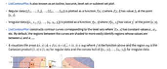
ListContourPlot 也被称为等值线、等曲线、水平集或次水平集图.
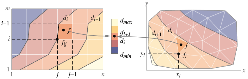
规则数据 {{f₁₁,…,f_1n},…,{f_m1,…,f_mn}} 绘制为函数 f[x,y]，其中在点 {x,y} 处 f[j,i] 的值为 f_ij.
不规则数据 {{x₁,y₁,f₁},…,{x_k,y_k,f_k}} 绘制为函数 f[x,y]，其中在点 {x,y} 处 f[x_i,y_i] 的值为 f_i.
ListContourPlot 构建对应于水平集的等高曲线，其中 f[x,y] 有常数 d₁、d₂ 等. 默认情况下，曲线之间的区域有阴影，以便更容易识别数值在 d_i 和 d_i+1 之间的区域.
该函数可视化区域，其中 f 为上述函数，且区域是规则数据的笛卡尔积，和不规则数据的 {{x₁,y₁},…,{x_n,y_n}} 的凸壳.

对于普通数据 {{f₁₁,…,f_1n},…,{f_m1,…,f_mn}}，值 f_ij 的位置被视为 . 使用选项 DataRange 可覆盖该认定.
默认情况下，对于色阶生成的输出，较大的值显示为较浅的颜色.
ListContourPlot 线性插值以给出平滑等高线.
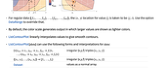
数据值 x_i、y_i 和 z_i 可以用以下形式给出：
x_i 实数值

Quantity[x_i,unit] 带单位的量
ListContourPlot[data] 可为 data 使用如下格式和解释：

	{<\|x_keyx₁,y_keyy₁,f_keyf₁\|>,…,<\|x_keyx_n,y_keyy_n,f_keyf_n\|>}	不规则三变量 {x_i,y_i,f_i}
	{{x₁,y₁},…,{x_n,y_n}}{f₁,…,f_n}	不规则三变量 {x_i,y_i,f_i}
	Dataset	作为正规数组的值
	NumericArray	作为正规数组的值
	QuantityArray	幅值
	SparseArray	作为正规数组的值

ListContourPlot[Tabular[…]cspec] 使用列规范 cspec 从表格对象中提取并绘制数值.
在绘制表格数据时，允许使用以下形式的列规范 cspec：

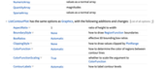
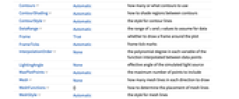
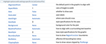
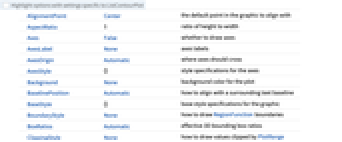
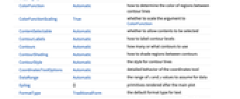
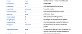
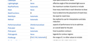
	{col_x,col_y,col_z}	绘制 z 列与 x 列和 y 列的对比图
	{{col_x1,col_y1,col_z1},{col_x2,col_y2,col_z2},…}	绘制列 z₁ 与列 x₁ 和列 y₁ 的对比图，绘制列 z₂ 与列 x₂ 和列 y₂ 的对比图等

ListContourPlot 的可选项与 Graphics 一样，可以有以下补充和修改： [所有选项的列表]

AspectRatio	1	长宽比
BoundaryStyle	None	如何绘制 RegionFunction 边界
BoxRatios	Automatic	有效的三维边框比率
ClippingStyle	None	如何绘制由 PlotRange 剪切的值
ColorFunction	Automatic	如何确定等高线之间的区域的着色
ColorFunctionScaling	True	是否按比例缩放 ColorFunction 的自变量
ContourLabels	Automatic	如何标记等高线的层次
Contours	Automatic	使用什么样的等高线及其数量
ContourShading	Automatic	怎样处理等高线之间区域的色调
ContourStyle	Automatic	等高线的样式
DataRange	Automatic	假设对数据所采用的 x 和 y 坐标值的范围
Frame	True	是否在图形周围绘制边框
FrameTicks	Automatic	边框刻度标记
InterpolationOrder	None	在数据点之间插值的函数的每个变量的多项式次数
LightingAngle	None	模拟光源的有效角度
MaxPlotPoints	Automatic	包含点的最大数量
Mesh	None	每个方向绘制网格线的数量
MeshFunctions	{}	如何确定网格线的放置
MeshStyle	Automatic	网格线的样式
Method	Automatic	插值和数据化简的方法
PerformanceGoal	$PerformanceGoal	优化的目标
PlotFit	None	如何对点进行曲线拟合
PlotFitElements	Automatic	绘图中显示的拟合元素
PlotInteractivity	$PlotInteractivity	是否允许出现互动元素
PlotLayout	Automatic	如何定位等高线
PlotLegends	None	等高线区域的图例
PlotRange	{Full,Full,Automatic}	包含 f 的范围或其它值
PlotRangeClipping	True	是否在绘图范围边界处进行剪切
PlotRangePadding	Automatic	需要填充的数值范围
PlotTheme	$PlotTheme	图线的整体主题
RegionFunction	(True&)	如何确定是否包含一个点
ScalingFunctions	None	如何缩放个别坐标

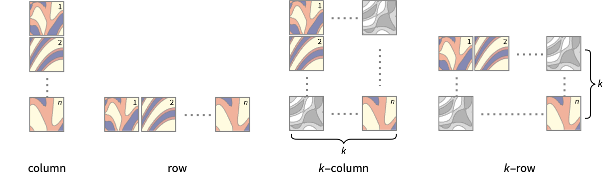
在多个绘图面板中显示单个等高线的 PlotLayout 可能设置包括：

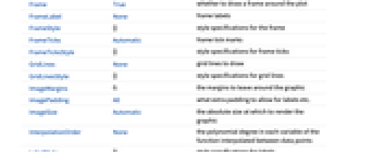
	"Column"	在一列面板中使用单独的等高线
	"Row"	在一行面板中使用单独的等高线
	{"Column",k},{"Row",k}	使用 k 列或行
	{"Column",UpTo[k]},{"Row",UpTo[k]}	使用至多 k 列或行

DataRange 确定数组 {{f₁₁,…,f_1n},…,{f_m1,…,f_mn}} 中值 f_ij 的 {x,y} 位置. 可能的设置包括：

	Automatic,All	在 x 中从 1 到 n 并在 y 中从 1 到 m 为统一变量
	{{x_min,x_max},{y_min,y_max}}	在 x 中从 x_min 到 x_max 并在 y 中从 y_min 到 y_max 为统一变量

ListContourPlot[{{a₁₁,a₁₂,a₁₃},…}] 的情况可以解释为规则数据和不规则数据. 设置 DataRange->Automatic 则解释为不规则 {{x₁,y₁,f₁},{x₂,y₂,f₂},…}，设置 DataRangeAll 则解释为规则 {{f₁₁,…,f_1n},…,{f_m1,…,f_mn}}.
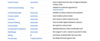
对于位于等高线层次之间的区域，在确定对区域如何着色的过程中，ListContourPlot 看起来首先处理 ContourShading 的设置，然后处理 ColorFunction 的设置.
ListContourPlot 对 SparseArray 对象起作用.
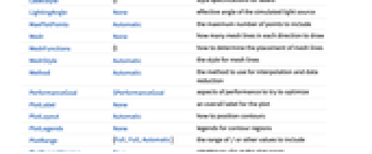
MeshFunctions 和 RegionFunction 中提供给函数的自变量是 x、y、f.
ColorFunction 默认下提供单个自变量，它由关于每对连续等高层的 f 的平均比例值给出.
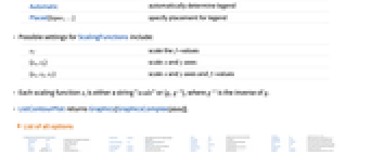
PlotLegends 的典型设置包括：
None 不使用图例

Automatic 自动确定图例

Placed[lspec,…] 指定图例位置
ScalingFunctions 的可能设置包括：
s_f f-值的比例

{s_x,s_y} 缩放 x 和 y 轴

{s_x,s_y,s_f} 缩放 x 和 y 轴以及 f-值
每个缩放函数 s_i 是字符串 "scale" 或 {g,g^-1}，其中 g^-1 是 g 的反函数.
ListContourPlot 返回 Graphics[GraphicsComplex[data]].

所有选项的列表

AlignmentPoint	Center	在图形内对齐的缺省点
AspectRatio	1	长宽比
Axes	False	是否绘制轴
AxesLabel	None	坐标轴标签
AxesOrigin	Automatic	坐标轴原点
AxesStyle	{}	坐标轴样式指定
Background	None	绘图的背景色
BaselinePosition	Automatic	如何与环绕文本基线对齐
BaseStyle	{}	图形的基本样式指定
BoundaryStyle	None	如何绘制 RegionFunction 边界
BoxRatios	Automatic	有效的三维边框比率
ClippingStyle	None	如何绘制由 PlotRange 剪切的值
ColorFunction	Automatic	如何确定等高线之间的区域的着色
ColorFunctionScaling	True	是否按比例缩放 ColorFunction 的自变量
ContentSelectable	Automatic	是否允许进行内容选择
ContourLabels	Automatic	如何标记等高线的层次
Contours	Automatic	使用什么样的等高线及其数量
ContourShading	Automatic	怎样处理等高线之间区域的色调
ContourStyle	Automatic	等高线的样式
CoordinatesToolOptions	Automatic	坐标工具的详细行为
DataRange	Automatic	假设对数据所采用的 x 和 y 坐标值的范围
Epilog	{}	主图形之后执行的图形指令
FormatType	TraditionalForm	文本的缺省样式类型
Frame	True	是否在图形周围绘制边框
FrameLabel	None	边框标签
FrameStyle	{}	边框的样式指定
FrameTicks	Automatic	边框刻度标记
FrameTicksStyle	{}	边框刻度的样式指定
GridLines	None	绘制的网格线
GridLinesStyle	{}	网格线的样式指定
ImageMargins	0.	图形周围的边幅
ImagePadding	All	为标签等额外填充内容
ImageSize	Automatic	图形的绝对尺寸
InterpolationOrder	None	在数据点之间插值的函数的每个变量的多项式次数
LabelStyle	{}	标签的样式指定
LightingAngle	None	模拟光源的有效角度
MaxPlotPoints	Automatic	包含点的最大数量
Mesh	None	每个方向绘制网格线的数量
MeshFunctions	{}	如何确定网格线的放置
MeshStyle	Automatic	网格线的样式
Method	Automatic	插值和数据化简的方法
PerformanceGoal	$PerformanceGoal	优化的目标
PlotFit	None	如何对点进行曲线拟合
PlotFitElements	Automatic	绘图中显示的拟合元素
PlotInteractivity	$PlotInteractivity	是否允许出现互动元素
PlotLabel	None	图形的一个整体标签
PlotLayout	Automatic	如何定位等高线
PlotLegends	None	等高线区域的图例
PlotRange	{Full,Full,Automatic}	包含 f 的范围或其它值
PlotRangeClipping	True	是否在绘图范围边界处进行剪切
PlotRangePadding	Automatic	需要填充的数值范围
PlotRegion	Automatic	填充的最后显示区域
PlotTheme	$PlotTheme	图线的整体主题
PreserveImageOptions	Automatic	当显示相同图形的新版本时，是否保存图形选项
Prolog	{}	主图形之前执行的图形指令
RegionFunction	(True&)	如何确定是否包含一个点
RotateLabel	True	是否在边框上旋转 y 标签
ScalingFunctions	None	如何缩放个别坐标
Ticks	Automatic	坐标轴标记
TicksStyle	{}	坐标轴标记的样式指定

范例

打开所有单元关闭所有单元

基本范例 (4)

从高度值数组产生等高线图：

给出数据明确的、、坐标：

使用图例在插值数据上生成等高线：

使用多面板布局同时显示多个数据集：

范围 (17)

数据 (8)

对于值组成的规则数据，和的数据范围采用整数值：

用 DataRange 提供明确的和的数据范围：

对由三元组组成的不规则数据，和的数据范围由数据推导出：

排除非实数数据的区域：

用 MaxPlotPoints 限制使用点的数量：

自动选择 PlotRange：

用 PlotRange 强调感兴趣的区域：

用 RegionFunction 限制不等式给出区域的密度：

表格数据 (1)

获取表格数据：

在 x 列和 y 列上绘制 f 列的阴影等值线图：

绘制多组柱状图，将图排列成一行：

为图表添加彩色条形图例：

演示 (8)

加上标签：

对高度值的密度着色：

显示图例：

标注等高线图：

在等高线间用指定的颜色：

用不同样式：

选用带有简单刻度和图例的主题样式：

使用多面板布局同时显示多个数据集：

使用列而不是行：

选项 (107)

AspectRatio (4)

默认情况下，ListContourPlot 使用相同的宽度和高度：

使用数值指定高宽比：

AspectRatioAutomatic 根据绘图范围确定比率:

AspectRatioFull 调整高度和宽度以紧密适合其他结构：

Axes (4)

默认情况下，ListContourPlot 使用边框而非轴：

使用轴而非边框：

使用 AxesOrigin 指定坐标区相交的位置：

单独打开每条轴：

AxesLabel (4)

默认情况下不绘制坐标轴标签：

在轴上放置一个标签：

指定轴标签：

使用单位作为标签：

AxesOrigin (2)

自动确定轴的位置：

为轴指定一个明确的原点：

AxesStyle (4)

更改轴的样式：

指定每条轴的样式：

对刻度和轴使用不同的样式：

对标签和轴使用不同的样式：

BoundaryStyle (4)

默认情况下不使用边界：

在等高线图周围绘制红色边界：

在 BoundaryStyle 中应用 RegionFunction 剪切的空间：

BoundaryStyle 在表面上应用跳跃变化：

ClippingStyle (4)

默认情况下不显示剪切区域：

着色剪切区域，就像表面的其余部分一样：

用红色填充剪切区域：

在表面上，上面剪切的区域用浅红色，下面剪切的区域用粉红色：

ColorFunction (2)

按尺度缩放的坐标着色：

在方向用已命名的颜色梯度着色：

ColorFunctionScaling (1)

如果等高值是负数，用蓝色着色，其它用红色：

ContourLabels (2)

对等高线增加标签：

在边框内标记值：

Contours (7)

使用 7 条等间隔的等高线：

自动选择等高线：

自动选择最多 5 条等高线：

绘制特定等高线：

绘制特定样式的特定等高线：

用函数产生等高线集合：

在 10％和 90％的百分位值的等高线：

ContourShading (4)

自动阴影在较低值处颜色较深，在较高值处颜色较浅：

用 None 仅显示等高线：

用颜色函数设置等高线间的阴影：

在等高线间用明确的颜色列表：

ContourStyle (5)

默认的等高线样式是部分透明的线条：

使用不透明的等值线：

用 None 不显示等高线：

红色等高线和虚线等高线交替：

用红虚线样式的等高线：

DataRange (4)

高度值数组的显示对应于每个方向上元素的数量：

重新调整取样空间：

三个一组可以视为、、坐标：

产生三个一组的数组：

强制解释为高度值的数组：

ImageSize (7)

使用有名称的尺寸，例如 Tiny、Small、Medium 和 Large：

指定绘图的宽度：

指定绘图的高度：

允许宽度和高度达到一定尺寸：

指定图形的宽度和高度，必要时用空白填充：

设置 AspectRatioFull 将填充可用空间：

对宽度和高度使用最大尺寸：

使用 ImageSizeFull 填充对象中的可用空间：

将图像大小指定为可用空间的一个比例：

InterpolationOrder (5)

等高线通常基于数据的一个线性插值：

用零阶或分段常量插值：

使用三阶样条插值，以拟合数据：

插值的次数从 0 到 5：

在有限数量的点下，线性插值不规则的数据：

设置 InterpolationOrder->1，不规则数据用自然相邻的插值：

MaxPlotPoints (4)

ListContourPlot 通常使用数据集合的所有点：

在每个方向显示使用点的数量：

MaxPlotPoints 在不规则数据上施加规则网格：

网格不会延伸出原始数据的凸壳：

Mesh (2)

显示最初和最后的取样网格线：

在每个方向上用 5 条网格线：

MeshFunctions (2)

在和方向上用 5 个网格线：

网格线层次对应于复数值函数的实部和虚部：

MeshStyle (2)

用红色网格线：

在方向用红色网格线，在方向用虚线网格线：

PerformanceGoal (2)

产生高质量的图形：

在牺牲质量的前提下强调性能：

PlotFit (4)

默认情况下，可以绘制出等值线图的许多细节：

对数据进行拟合可得到更平滑的等值线图：

用二次曲面拟合数据：

用 KernelModelFit 近似数据：

PlotInteractivity (2)

默认情况下，等值线图含有交互式工具条：

禁用互动功能：

PlotLayout (3)

使用共用轴将每个等高线放在单独的面板中：

使用行而非列：

使用多列或多行：

首选满列或满行：

PlotLegends (6)

默认情况下，不使用图例：

包括图例：

图例自动使用与密度图线相同的颜色：

使用 Placed 改变图例位置：

使用 BarLegend 定制图例：

图例自动选择添加标签的等高线：

对全部等高线添加标签：

PlotRange (3)

自动计算的范围：

用所有点计算范围：

用一个明确的范围来强调特色：

PlotTheme (1)

使用黑白方案：

改变色调：

添加图例，并且改变等高线样式：

RegionFunction (4)

绘制上的区域：

区域取决于 DataRange：

区域可以互不相连：

使用条件的任意逻辑组合：

ScalingFunctions (9)

默认情况下，绘图在每个方向上都使用线性刻度：

在方向使用对数刻度：

在方向使用线性刻度，在顶部显示更小的数字：

在方向上使用倒数刻度：

在和方向使用不同的刻度：

不改变轴的情况下翻转轴：

使用由函数和反函数定义的刻度：

Ticks 和 GridLines 的位置是自动安排的：

PlotRange 是自动安排的：

应用 (2)

概率密度函数的等高线图：

与实际的密度函数比较：

医药数据的等高线图：

属性和关系 (15)

ListContourPlot 相似于 ListDensityPlot，但有带状的离散颜色：

在 ListContourPlot 和 ListPlot3D 中，将视为和的函数：

数据在每对、仅对应一个值：

这个数据在每对、上对应有 2 个值：

对离散数据的数组运用 ArrayPlot：

用 MatrixPlot 绘制矩阵的结构图形：

用 ReliefPlot 处理对应于医疗和地理数据的矩阵：

用 GeoContourPlot 绘制地理数据：

用 ListContourPlot3D 产生四维数据的等高面：

对函数用 ContourPlot：

用 ListPointPlot3D 显示三维点：

用 ListDensityPlot 创建连续数据的密度：

用 ListPlot3D 创建连续数据的表面：

用 ListLogPlot、ListLogLogPlot 和 ListLogLinearPlot 处理对数图形：

用 ListPolarPlot 处理极坐标图形：

用 DateListPlot 显示时间上的数据：

用 ParametricPlot3D 处理三维参数曲线和表面：

可能存在的问题 (2)

外观取决于数据源：

一个 ×3 矩阵默认情况下视为三个一组的列表：

用 DataRange->All 强制解释为值的矩阵：

或提供一个明确的数据范围来强制解释为值的矩阵：

Top

	x_i	实数值
	Quantity[x_i,unit]	带单位的量

	None	不使用图例
	Automatic	自动确定图例
	Placed[lspec,…]	指定图例位置

	s_f	f-值的比例
	{s_x,s_y}	缩放 x 和 y 轴
	{s_x,s_y,s_f}	缩放 x 和 y 轴以及 f-值