


Plot
詳細とオプション
- Plotは関数プロットあるいは関数のグラフとしても知られている.
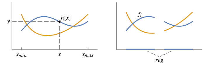
- Plotはプロットされている領域の x の値のところで f を評価し,点{x,f[x]}を繋いで x に従って f がどのように変化するかを示す曲線を描く.これは,曲線
 を可視化する.
- fiが実数あるいはQuantity以外に評価される任意の x のところにはギャップが残される.
- 極限 xminおよび xmaxは,実数あるいはQuantity式でよい.
- 領域 reg は1Dの任意のRegionQオブジェクトでよい.
- Plotは,実質的にBlockを使って変数 x を局所的なものとして扱う.
- Plotは属性HoldAllを持ち,x に特定の数値を割り当てた後で f を評価する.
- 場合によっては,x に特定の数値が割り当てられる前にEvaluateを使って f を記号的に評価する方が効率的なこともある.
- fiには次のラッパー w が使える.
-
Annotation[fi,label] fiについての注釈を与える Button[fi,action] fiの曲線がクリックされたときに action を評価する Callout[fi,label] コールアウトで関数にラベルを付ける Callout[fi,label,pos] コールアウトを相対位置 pos に置く EventHandler[fi,events] fiについての一般的なイベントハンドラを定義する Highlighted[fi,effect] 効果を付けて fiを動的にハイライトする Highlighted[fi,Placed[effect,pos]] 位置 pos で効果を付けて fiを静的にハイライトする Hyperlink[fi,uri] 関数をハイパーリンクにする Labeled[fi,label] 関数にラベルを付ける Labeled[fi,label,pos] ラベルを相対位置 pos に置く Legended[fi,label] 凡例で関数を識別する PopupWindow[fi,cont] 関数にポップアップウィンドウを付ける StatusArea[fi,label] マウスオーバーの際にステータスエリアに表示する Style[fi,styles] 関数を指定のスタイルで表示する Tooltip[fi,label] 関数にツールチップを付ける Tooltip[fi] 関数をツールチップとして使う - ラッパー w は複数のレベルで適用することができる.
-
w[fi] fiを囲む w[{f1,…}] fiの集合を囲む w1[w2[…]] ネストしたラッパーを使う - Callout,Labeled,Placedには次の位置 pos を使うことができる.
-
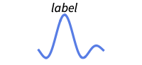
Above 曲線の上の位置 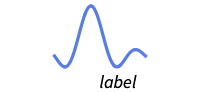
Below 曲線の下の位置 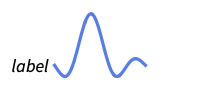
Before 曲線の前の位置 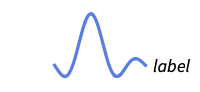
After 曲線の後ろの位置 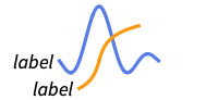
Start 各曲線の開始位置 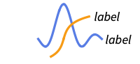
End 各曲線の終了位置 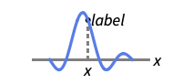
x 位置 x における曲線の近く 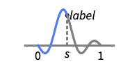
Scaled[s] 曲線に沿ってスケールされた位置 s 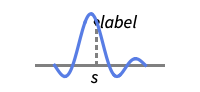
{s,Above} 曲線に沿った位置 s の相対的な位置の上 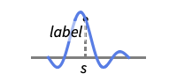
{s,Below} 曲線に沿った位置 s の相対的な位置の下 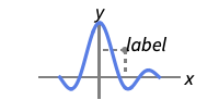
{pos,epos} 曲線の相対的な位置 pos に置かれたラベル内の epos - Plotには,Graphicsと同じオプションに以下の追加・変更を加えたものが使える. [全オプションのリスト]
- ClippingStyleの可能な設定
-

Automatic 切り取られた部分に点線を使う 
None 曲線の切り取られた部分を省略する 
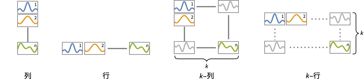
style 切り取られた部分に style を使う - 次は,複数のプロットパネルのそれぞれに単一の曲線を表示するPlotLayoutの可能な設定である.
-
"Column" パネルの列に別々の曲線を使う "Row" パネルの行に別々の曲線を使う {"Column",k},{"Row",k} k 列(または行)を使う {"Column",UpTo[k]},{"Row",UpTo[k]} 最高で k 列(または行)を使う - デフォルト設定のExclusions->AutomaticとExclusionsStyle->Noneでは,Plotが不連続性や特異点を検知したところで曲線が途切れる.Exclusions->Noneとすると,不連続性や特異点があっても曲線は繋がれる.
- Exclusions->{x1,x2,…}はExclusions->{x==x1,x==x2,…}に等しい.
- HighlightedとPlotHighlightingの使用可能なハイライト効果には以下がある.
-
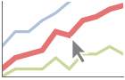
style 指定された曲線をハイライトする 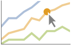
"Ball" 曲線上の指定された点をハイライトしてこれにラベルを付ける 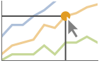
"Dropline" 軸までのドロップラインを付けることで曲線上の指定された点をハイライトしてこれにラベルを付ける 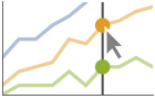
"XSlice" 垂直スライスに沿ったすべての点をハイライトしてこれにラベルを付ける 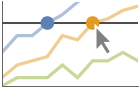
"YSlice" 水平スライスに沿ったすべての点をハイライトしてこれにラベルを付ける 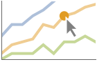
Placed[effect,pos] 指定の位置 pos を静的にハイライトする - 位置指定 pos のハイライトには以下がある.
-
x, {x} {x,y}における効果.y は自動的に選択される {x,y} {x,y}における効果 {pos1,pos2,…} 複数の位置 posi - PlotLegendsの典型的な設定には,次が含まれる.
-
None 凡例なし Automatic 凡例を自動的に決定する "Expressions" f1, f2, …を凡例ラベルとして用いる {lbl1,lbl2,…} lbl1, lbl2, …を凡例ラベルとして用いる Placed[lspec,…] 凡例の配置を指定する - PlotStylesty は,各曲線に使用するスタイルを指定する.設定可能な値には次が含まれる.
-
{sty1,sty2,…} データ集合に対するスタイルの列 <"key"val,…> データの異なるレベルに対するスタイル要素 - 使用可能なキーは次の通りである.
-
"Base" すべての fi に対する全体的なスタイル "Functions" 各 fi に対するスタイル styi のリスト - ColorData["DefaultPlotColors"]は,PlotStyleで使われるデフォルトの色のシーケンスを与える.
- Plotは,まず,f をPlotPointsで指定された等間隔のサンプル点の数で評価する.次に,適応的アルゴリズムを使用し,指定の区間を最大MaxRecursion回まで部分分割して追加のサンプル点を選択する.
- 有限個のサンプル点を使用した場合には,Plotが f の特徴を見逃す可能性があることを認識しておいてほしい.結果を確認する方法として,PlotPointsやMaxRecursionを増加する方法がある.
- 曲線に影響するテーマ
-

"ThinLines" 細いプロット線 
"MediumLines" 中くらいのプロット線 
"ThickLines" 太いプロット線 - MeshFunctionsおよびRegionFunctionの関数に渡される引数は,x および y である.デフォルトで,ColorFunctionの関数にはこれらの引数のスケールされたバージョンが渡される.
- 次はScalingFunctionsの可能な設定である.
-
sy y 軸をスケールする {sx,sy} x 軸と y 軸をスケールする - 各スケーリング関数 siは"scale"または{g,g-1}のどちらかである.g-1は g の逆である.
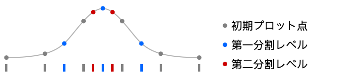
全オプションのリスト
例題
すべて開く すべて閉じる例 (5)
Plot[Sin[x], {x, 0, 6Pi}]Plot[{Sin[x], Sin[2x], Sin[3x]}, {x, 0, 2Pi}, PlotLegends -> "Expressions"]Plot[{Sin[x], Cos[x]}, {x, 0, 2Pi}, PlotLabels -> "Expressions"]Plot[2Sin[x] + x, {x, 0, 15}, Filling -> Bottom]Plot[{Sin[x] + x / 2, Sin[x] + x}, {x, 0, 10}, Filling -> {1 -> {2}}]自動的に透過色を使って複数の塗り潰された曲線をプロットする:
Plot[Evaluate[Table[BesselJ[n, x], {n, 4}]], {x, 0, 10}, Filling -> Axis]スコープ (33)
サンプリング (10)
関数の変化が速いときにはより多くの点がサンプルとして取られる:
Plot[Sin[30Sin[x]], {x, 0, 10}]Plot[1 / x, {x, -1, 1}]Plot[Sqrt[x], {x, -1, 1}]Plot[Floor[Sqrt[x]], {x, 0, 100}]Exclusions->Noneを使って連結線を描く:
Plot[Floor[Sqrt[x]], {x, 0, 100}, Exclusions -> None]PlotPointsとMaxRecursionを使って適応的サンプリングを制御する:
Grid@Table[Plot[Sin[x], {x, 0, 15}, PlotPoints -> pp, MaxRecursion -> mr], {mr, {0, 1, 2}}, {pp, {5, 10}}]PlotRangeを使って関心領域に焦点を当てる:
{Plot[x ^ 4 - x ^ 2 + 1, {x, -2, 2}], Plot[x ^ 4 - x ^ 2 + 1, {x, -2, 2}, PlotRange -> {0, 2}]}𝒟 = ImplicitRegion[x ≤ -1∨x ≥ 1, {x}];Plot[Sin[x], {x}∈𝒟]MeshRegionを使って領域を指定する:
𝒟 = MeshRegion[{{-2}, {-1}, {-1 / 2}, {1 / 2}, {1}, {2}}, Line[{{1, 2}, {3, 4}, {5, 6}}]];Plot[x ^ 3 + 1, {x}∈𝒟]Plot[Sinc[x], {x, -Infinity, Infinity}]ScalingFunctionsを使って軸をスケールする:
Plot[Abs[Gamma[z]], {z, -4, 8}, ScalingFunctions -> "Log"]ラベルと凡例 (11)
Labeledで曲線にラベルを付ける:
Plot[Evaluate@Table[Labeled[x ^ n, x ^ n], {n, 1, 3}], {x, -3, 3}]Table[Plot[Labeled[Cos[x], Cos[x], p], {x, 0, 2Pi}, PlotLabel -> p], {p, {Above, Below, Before, After}}]PlotLabelsで曲線にラベルを付ける:
Plot[{Sin[x], Sin[2x]}, {x, 0, 6}, PlotLabels -> {Sin[x], Sin[2x]}]
Plot[Labeled[Sin[x], "sin(x)", 3], {x, 0, 2π}]Plot[Labeled[Sin[x], "sin(x)", Scaled[0.25]], {x, 0, 2π}]Plot[Labeled[Sin[x], Sin[x], {Scaled[0.25], Above}], {x, 0, 2π}]Calloutで自動的に曲線にラベルを付ける:
Plot[{Callout[n ^ Sin[n], n ^ Sin[n]], Callout[n, n]}, {n, 0, 20}]Plot[Callout[n ^ Sin[n], "label", Above], {n, 1, 10}]Plot[Callout[n ^ Sin[n], "label", 2], {n, 1, 10}]Plot[{Sin[x], Cos[x]}, {x, 0, 2π}, PlotLegends -> {Sin[x], Cos[x]}]Legendedを使って特定の曲線に凡例を付ける:
Plot[{Sin[x], Legended[Mean[{Sin[x], Cos[x]}], "average"], Cos[x]}, {x, 0, 2π}]Placedを使って凡例の位置を変える:
Plot[{Sin[x], Legended[Mean[{Sin[x], Cos[x]}], Placed["average", Below]], Cos[x]}, {x, 0, 2π}]通常,曲線にはマウスオーバーの際に座標を表示するインタラクティブなコールアウトがある:
Plot[Sin[x] + x, {x, 0, 10}]特定のラッパーあるいはツールチップのようなインタラクションを含めてインタラクティブな機能をオフにする:
Plot[Callout[Sin[x] + x, "hello", 6], {x, 0, 10}]{Plot[{Sin[x] / x, Cos[x] / x}, {x, 0, 10}, PlotHighlighting -> "Dropline"], Plot[{Sin[x] / x, Cos[x] / x}, {x, 0, 10}, PlotHighlighting -> "XSlice"]}Highlightedを使ってプロット中の特定の点を強調する:
Plot[Highlighted[Sinc[x], Placed["Ball", 2]], {x, 0, 10}]Plot[Highlighted[Sinc[x], Placed["Ball", {{2}, {7}}]], {x, 0, 10}]プレゼンテーション (12)
Plot[{x ^ (1 / 4), x ^ (3 / 4), x ^ (3 / 2), x ^ (7 / 2)}, {x, 0, 2}]Plot[{x ^ (1 / 4), x ^ (3 / 4), x ^ (3 / 2), x ^ (7 / 2)}, {x, 0, 2}, PlotStyle -> {Thick, Automatic, Red, Dashed}]Plot[{x ^ (1 / 4), x ^ (3 / 4), x ^ (3 / 2), x ^ (7 / 2)}, {x, 0, 2}, PlotStyle -> {Thick, Automatic, Red, Dashed}, PlotLegends -> Automatic]Plot[Sin[x], {x, 0, 2Pi}, AxesLabel -> {x, y}, PlotLabel -> Sin[x]]Plot[{x, x ^ 2, x ^ 3}, {x, -2, 2}, PlotLabels -> Automatic]Plot[Labeled[x ^ 4 - 25 x ^ 2 + 20 x + 15, {"abs max", "abs min", "rel max", "rel min"}, {Above, Below, 0.5, 3.5}], {x, -5, 5}]各曲線にインタラクティブなTooltipを加える:
Plot[{Tooltip[Sin[x]], Tooltip[Sin[2x]]}, {x, 0, 2Pi}]Plot[{Sin[x], Cos[x]}, {x, 0, 2Pi}, Filling -> Axis]Plot[{Sin[x], Cos[x]}, {x, 0, 2Pi}, PlotTheme -> "Marketing"]Plot[Sin[x], {x, 0, 2Pi}, Mesh -> 20]Plot[Sin[x], {x, 0, 2Pi}, Mesh -> 10, MeshShading -> {Red, None, Blue}]Plot[{Sin[x] / x, 1 / x, -1 / x}, {x, -Infinity, Infinity}]Plot[{Sin[t], Cos[t]}, {t, 0, 4Pi}, PlotLayout -> "Row"]Plot[{Sin[t], Cos[t]}, {t, 0, 4Pi}, PlotLayout -> "Column"]Plot[{BesselJ[0, x], BesselJ[1, x], BesselJ[2, x], BesselJ[3, x], BesselJ[4, x], BesselJ[5, x]}, {x, -20, 20}, PlotLayout -> {"Row", 2}]オプション (132)
AspectRatio (1)
Axes (2)


AxesLabel (2)
Plotで指定された変数に基づいたラベルを使う:
Plot[Sinc[u], {u, 0, 10}, AxesLabel -> Automatic]Plot[Sinc[x], {x, 0, 10}, AxesLabel -> {x, Sinc[x]}]AxesOrigin (2)

AxesStyle (3)
Plot[Sinc[x], {x, 0, 10}, AxesStyle -> Red]Plot[Sinc[x], {x, 0, 10}, AxesStyle -> {Thick, Blue}]Plot[Sinc[x], {x, 0, 10}, AxesStyle -> Blue, TicksStyle -> Red]Plot[Sinc[x], {x, 0, 10}, AxesStyle -> Blue, LabelStyle -> Red]BaselinePosition (1)

ClippingStyle (5)
Plot[Sin[x] / x ^ 2, {x, -10, 10}, ClippingStyle -> None]Plot[Sin[x] / x ^ 2, {x, -10, 10}, ClippingStyle -> Automatic]Plot[Sin[x] / x ^ 2, {x, -10, 10}, ClippingStyle -> Red]Plot[Sin[x] / x ^ 2, {x, -10, 10}, ClippingStyle -> {Red, Thick}]Plot[Sin[x] / x ^ 2, {x, -10, 10}, ClippingStyle -> Directive[Red, Thick]]ColorFunction (5)


{Plot[Sinc[x], {x, 0, 10}, ColorFunction -> Function[{x, y}, Hue[y]]], Plot[Sinc[x], {x, 0, 10}, ColorFunction -> Function[{x, y}, Hue[x]]]}Plot[Sinc[x], {x, 0, 10}, ColorFunction -> "DarkRainbow"]
Plot[Sinc[x], {x, 0, 10}, ColorFunction -> Function[{x, y}, If[y > 0, Red, StandardBlue]], ColorFunctionScaling -> False, PlotStyle -> Thick]Plot[Sin[x], {x, 0, 2Pi}, ColorFunction -> Function[{x, y}, Hue[y]], Filling -> Axis]ColorFunctionは,曲線の色付けに関してはPlotStyle より優先順位が高い:
Plot[Sinc[x], {x, 0, 10}, ColorFunction -> "DarkRainbow", PlotStyle -> Directive[Red, Thick]]ColorFunctionScaling (3)
左側では引数のスケーリングは行わず,右側は自動スケーリングを使う:
Table[Plot[Sin[4Pi x], {x, 0, 1 / 2}, PlotStyle -> Thick, ColorFunction -> Function[{x, y}, Hue[x]], ColorFunctionScaling -> cf], {cf, {False, True}}]
Plot[Sinc[x], {x, 0, 10}, ColorFunction -> Function[{x, y}, If[y > 0, Red, StandardBlue]], ColorFunctionScaling -> False, PlotStyle -> Thick]
Plot[Sin[2x], {x, 0, 2Pi}, ColorFunction -> Function[{x, y}, Hue[x, 1, Abs[y]]], ColorFunctionScaling -> {True, False}, PlotStyle -> Thick]Epilog (2)
以下は,結果のグラフィックスにグラフィックスオブジェクトを挿入する:
Plot[Sin[x], {x, 0, 2Pi}, Epilog -> {PointSize[0.04], Point[{0, 0}], Point[{Pi, 0}], Point[{2Pi, 0}]}]点が曲線に属するのかどうかを示すための特別のマーカーを挿入する:
Plot[Floor[x], {x, -2, 3}, Epilog -> {Table[Disk[{i, i}, Offset[2.]], {i, -2, 2}], Table[{EdgeForm[StandardGray], White, Disk[{i + 1, i}, Offset[2]]}, {i, -2, 2}]}]EvaluationMonitor (3)
Plotによって見本として抽出された値のリストを求める:
Reap[Plot[Sin[x], {x, 0, 10}, EvaluationMonitor :> Sow[x]];]//Shortdata = Reap[ Plot[ Sin[x], {x, 0, 2Pi}, EvaluationMonitor :> Sow[{x, Sin[x]}]] ][[-1, 1]];ListPlot[data , Filling -> Axis]Block[{k = 0}, Plot[Sin[x], {x, 0, 2Pi}, EvaluationMonitor :> k++];k]Exclusions (7)
これは,除外するものの計算に自動的な方法,この場合は区分関数を使っている:
Plot[Floor[x ^ 2], {x, 0, 5}]Plot[Im[Sqrt[-1 + I (y + 1)]], {y, -2, 0}]Plot[Im[Sqrt[-1 + I (y + 1)]], {y, -2, 0}, Exclusions -> None]Plot[Tan[x], {x, -2, 2}, Exclusions -> {-Pi / 2, Pi / 2}]Plot[1 / (x ^ 3 - x + 1), {x, -2, 2}, Exclusions -> {x ^ 3 - x + 1 == 0}]Plot[Tan[x ^ 3 - x + 1] + 1 / (x + 3Exp[x]), {x, -2, 2}, Exclusions -> {Cos[x ^ 3 - x + 1] == 0, x + 3Exp[x] == 0}]Plot[Floor[Tan[x]], {x, -2, 2}, Exclusions -> {Automatic, Cos[x] == 0}]ExclusionsStyle (2)
Filling (7)
Table[Plot[Sin[x], {x, 0, 2Pi}, Filling -> f], {f, {Axis, Top, Bottom, 0.3}}]Plot[{Sin[x], Cos[x]}, {x, 0, 2Pi}, Filling -> Axis]
Plot[{Sin[x], Cos[x]}, {x, 0, 2Pi}, Filling -> {1 -> Axis}]Plot[{Sin[x], Cos[x]}, {x, 0, 2Pi}, Filling -> {1 -> {2}}]Plot[{Sin[x], Cos[x]}, {x, 0, 2Pi}, Filling -> {1 -> {{2}, StandardGray}}]
Plot[{Sin[x], Cos[x]}, {x, 0, 2Pi}, Filling -> {1 -> {1 / 2, StandardGray}}]曲線1と2の間を塗り潰す.1が2の下のときは黄色,1が2の上のときは緑を使う:
Plot[{Sin[x], Cos[x]}, {x, 0, 2Pi}, Filling -> {1 -> {{2}, {StandardGray, StandardGreen}}}]FillingStyle (4)
Table[Plot[Sin[x], {x, 0, 2Pi}, Filling -> Axis, FillingStyle -> c], {c, {Red, StandardGreen, StandardBlue, StandardYellow}}]Plot[{Sin[x], Cos[x]}, {x, 0, 2Pi}, Filling -> Axis, FillingStyle -> Directive[Opacity[0.5], Orange]]
Plot[Sin[x], {x, 0, 2Pi}, Filling -> Axis, FillingStyle -> {Red, Blue}]ColorFunctionから入手した変数の塗り潰しスタイルを使う:
Plot[Sin[x], {x, 0, 2Pi}, ColorFunction -> Function[{x, y}, Hue[y]], Filling -> Axis, FillingStyle -> Automatic]ImageSize (6)
Tiny,Small,Medium,Largeのような名前付きのサイズを使う:
{Plot[Sin[x], {x, 0, 10}, ImageSize -> Tiny], Plot[Sin[x], {x, 0, 10}, ImageSize -> Small]}{Plot[Sin[x], {x, 0, 10}, ImageSize -> 150], Plot[Sin[x], {x, 0, 10}, AspectRatio -> 2, ImageSize -> 150]}{Plot[Sin[x], {x, 0, 10}, ImageSize -> {Automatic, 150}], Plot[Sin[x], {x, 0, 10}, AspectRatio -> 2, ImageSize -> {Automatic, 150}]}{Plot[Sin[x], {x, 0, 10}, ImageSize -> UpTo[200]], Plot[Sin[x], {x, 0, 10}, AspectRatio -> 2, ImageSize -> UpTo[200]]}グラフィックスの幅と高さを指定し,必要な場合はスペースで充填する:
Plot[Sin[x], {x, 0, 10}, ImageSize -> {200, 200}, Background -> StandardOrange]AspectRatioFullとすると使用可能なスペースが埋められる:
Plot[Sin[x], {x, 0, 10}, AspectRatio -> Full, ImageSize -> {200, 200}, Background -> StandardOrange]ImageSizeFullを使ってオブジェクト内の使用可能なスペースを塗り潰す:
Framed[Pane[Plot[Sin[x], {x, 0, 10}, ImageSize -> Full, Background -> StandardOrange], {200, 100}]]Framed[Pane[Plot[Sin[x], {x, 0, 10}, ImageSize -> Scaled[0.5], Background -> StandardOrange], {200, 100}]]LabelingSize (3)
Plot[{Sin[x] + x, x Log[x]}, {x, 0, 5}, PlotLabels -> {"barcarole", "perilously"}]Plot[{Sin[x] + x, x Log[x]}, {x, 0, 5}, PlotLabels -> {[image], [image]}]Plot[{Sin[x] + x, x Log[x]}, {x, 0, 5}, PlotLabels -> {"barcarole", "perilously"}, LabelingSize -> 30]Plot[{Sin[x] + x, x Log[x]}, {x, 0, 5}, PlotLabels -> {[image], [image]}, LabelingSize -> 50]MaxRecursion (2)
Plot[Sin[1 / x], {x, 0.001, 0.1}, Mesh -> All]MaxRecursionの各レベルが最初のメッシュをより細かいメッシュに分割する:
Table[ Plot[Sin[1 / x], {x, 0.001, 0.1}, MaxRecursion -> i, Mesh -> All, Ticks -> None], {i, {0, 3, 6}}]Mesh (3)
{Plot[Sin[x], {x, 0, 2Pi}, Mesh -> Full],
	Plot[Sin[x], {x, 0, 2Pi}, Mesh -> All]}
Plot[Sin[x], {x, 0, 2Pi}, Mesh -> 20]
Plot[Sin[x], {x, 0, 2Pi}, Mesh -> {Range[0, 2Pi, Pi / 4]}, MeshStyle -> PointSize[Medium]]MeshFunctions (2)


Table[Plot[Tan[x], {x, 0, Pi / 2}, MeshFunctions -> {f}, Mesh -> 20], {f, {Function[{x, y}, x], Function[{x, y}, y]}}] 方向に赤で5つのメッシュレベルを,
 方向に青で10のメッシュレベルを示す:
Plot[Tan[x], {x, 0, Pi / 2}, Mesh -> {5, 10}, MeshFunctions -> {#1&, #2&}, MeshStyle -> {Directive[PointSize[Medium], Red], Blue}]MeshShading (6)

Plot[Sin[x], {x, 0, 2Pi}, Mesh -> 10, MeshFunctions -> {#1&}, MeshShading -> {Red, Blue}]Noneを使って線分を消去する:
Plot[Sin[x], {x, 0, 2Pi}, Mesh -> 10, MeshFunctions -> {#1&}, MeshShading -> {Red, None}]MeshShadingはPlotStyleとともに使うことができる:
Plot[Sin[x], {x, 0, 2Pi}, Mesh -> 10, PlotStyle -> Thick, MeshFunctions -> {#1&}, MeshShading -> {Red, Blue}]曲線のスタイルに関しては,MeshShadingはPlotStyleよりも優先順位が高い:
Plot[Sin[x], {x, 0, 2Pi}, Mesh -> 10, PlotStyle -> Green, MeshFunctions -> {#1&}, MeshShading -> {Red, Blue}]MeshShadingをAutomaticにして線分にPlotStyleを使う:
Plot[Sin[x], {x, 0, 10}, Mesh -> 10, PlotStyle -> Directive[Thick, Yellow], MeshFunctions -> {#1&}, MeshShading -> {Red, Automatic}]MeshShadingはColorFunctionとともに使うことができる:
Plot[Sin[x], {x, 0, 10}, Mesh -> 10, PlotStyle -> Thick, MeshFunctions -> {#1&}, MeshShading -> {StandardGray, Automatic},
	ColorFunction -> Function[{x, y}, Hue[x]]]
MeshStyle (4)
Plot[Sin[x], {x, 0, 2Pi}, Mesh -> 10, MeshStyle -> Automatic]
Plot[Sin[x], {x, 0, 2Pi}, Mesh -> 10, MeshStyle -> Red]

Plot[Sin[x], {x, 0, 2Pi}, Mesh -> 10, MeshStyle -> {Red, Blue}, MeshFunctions -> {#1&, #2&}]
Plot[Sin[x], {x, 0, 2Pi}, Mesh -> 10, MeshStyle -> Directive[PointSize[Large], Red]]PerformanceGoal (2)
PlotHighlighting (9)
プロットには,デフォルト設定がPlotHighlightingAutomaticのインタラクティブな座標コールアウトが付いている:
Plot[{Sin[x] + x, Sin[x]x}, {x, 0, 10}]PlotHighlightingNoneを使ってプロット全体のハイライト効果をオフにする:
Plot[{Sin[x] + x, Sin[x]x}, {x, 0, 10}, PlotHighlighting -> None]Highlighted[…,None]を使って単一の曲線のハイライト効果をオフにする:
Plot[{Sin[x] + x, Highlighted[Sin[x]x, None]}, {x, 0, 10}]任意のグラフィックス指示子を使い,マウスオーバーして曲線をハイライトする:
Plot[{Sin[x] + x, Sin[x]x}, {x, 0, 10}, PlotHighlighting -> Directive[Red, Dashed, DropShadowing[]]]Plot[Sin[x] + x, {x, 0, 10}, PlotHighlighting -> "Ball"]Plot[Highlighted[Sin[x] + x, Placed["Ball", 7]], {x, 0, 10}]曲線にマウスオーバーしてラベルと軸へのドロップラインでハイライトする:
Plot[Sin[x] + x, {x, 0, 10}, PlotHighlighting -> "Dropline"]Plot[Highlighted[Sin[x] + x, Placed["Dropline", 7]], {x, 0, 10}]プロットにマウスオーバーして  の位置に対応する
 の値を示すスライスでハイライトする:
Plot[{Sin[x] + x, Cos[x] + x}, {x, 0, 10}, PlotHighlighting -> "XSlice"]
Plot[Highlighted[{Sin[x] + x, Cos[x] + x}, Placed["XSlice", 6]], {x, 0, 10}]プロットにマウスオーバーして  の位置に対応する
 の値を示すスライスでハイライトする:
Plot[{Sin[x] + x, Cos[x] + x}, {x, 0, 10}, PlotHighlighting -> "YSlice"]
Plot[Highlighted[{Sin[x] + x, Cos[x] + x}, Placed["YSlice", 6]], {x, 0, 10}]マウスカーソルの  の位置に最も近い曲線上の点を示す成分を使う:
Plot[{Sin[x] + x, Cos[x] + x}, {x, 0, 10}, PlotHighlighting -> "XNearestPoint"]Plot[{Sin[x] + x, Cos[x] + x}, {x, 0, 10}, PlotHighlighting -> {"XNearestPoint", <|"Style" -> StandardGray|>}]Plot[Sin[x] + x, {x, 0, 10}, PlotHighlighting -> "XYLabel"]Calloutオプションを使ってラベルの外観を変える:
Plot[Sin[x] + x, {x, 0, 10}, PlotHighlighting -> {"XYLabel", <|"Appearance" -> "Corners", "CalloutMarker" -> "Circle"|>}]Plot[Sin[x] + x, {x, 0, 10}, PlotHighlighting -> {{"XNearestPoint", <|"Style" -> StandardGray|>}, {"XYLabel", <|"Appearance" -> "Corners", "CalloutMarker" -> "Circle"|>}}]PlotInteractivity (4)
デフォルトで,プロットにはインタラクティブなハイライト機能がある:
Plot[x + Sin[x], {x, 0, 20}]Plot[x + Sin[x], {x, 0, 20}, PlotInteractivity -> False]Plot[Tooltip[x + Sin[x], "hello"], {x, 0, 20}, PlotInteractivity -> False]与えたインタラクティブ要素は有効にして,自動のものを無効にする:
Plot[Tooltip[x + Sin[x], "hello"], {x, 0, 20}, PlotInteractivity -> <|"User" -> True, "System" -> False|>]PlotLabel (1)
PlotLabels (5)
Plot[{Sin[x], Cos[x]}, {x, 0, 2π}, PlotLabels -> {"sine", "cosine"}]Plot[{Sin[x], Cos[x]}, {x, 0, 2π}, PlotLabels -> Placed[{"sine", "cosine"}, Above]]Plot[{Sin[x], Cos[x]}, {x, 0, 2π}, PlotLabels -> {Placed["sine", Below], Placed["cosine", Above]}]PlotLabels->"Expressions"は関数を曲線のラベルとして使う:
Plot[{Sin[x], Cos[x]}, {x, 0, 2π}, PlotLabels -> "Expressions"]Plot[{Sin[x], Cos[x]}, {x, 0, 2π}, PlotLabels -> {Callout["sin", {Scaled[0.25], Above}], Callout["cos", {Scaled[0.5], Below}]}]Noneを使ってラベルを付けないようにする:
Plot[{Sin[x], Cos[x]}, {x, 0, 2π}, PlotLabels -> {"sine", None}]PlotLayout (2)
Plot[{Sin[x], Sin[2 x], Sin[3 x]}, {x, 0, 10}, PlotLayout -> "Column"]Plot[{Sin[x], Sin[2 x], Sin[3 x]}, {x, 0, 10}, PlotLayout -> "Row"]Plot[{BesselJ[0, x], BesselJ[1, x], BesselJ[2, x], BesselJ[3, x], BesselJ[4, x], BesselJ[5, x]}, {x, -20, 20}, PlotLayout -> {"Column", 4}]Plot[{BesselJ[0, x], BesselJ[1, x], BesselJ[2, x], BesselJ[3, x], BesselJ[4, x], BesselJ[5, x]}, {x, -20, 20}, PlotLayout -> {"Column", UpTo[4]}]PlotLegends (7)
Plot[{Sin[x], Cos[x]}, {x, 0, 10}]Plot[{Sin[x], Cos[x]}, {x, 0, 10}, PlotLegends -> "Expressions"]Plot[{Sin[x], Cos[x]}, {x, 0, 10}, PlotLegends -> "Placeholder"]Plot[{Sin[x], Cos[x]}, {x, 0, 10}, PlotLegends -> {"one", "two"}]PlotLegendsは自動的にPlotStyleの値を拾う:
Plot[{Sin[x], Cos[x]}, {x, 0, 10}, PlotStyle -> {Red, Blue}, PlotLegends -> "Placeholder"]Placedを使って凡例の置き方を決める:
Plot[{Sin[x], Cos[x]}, {x, 0, 10}, PlotStyle -> {Red, Blue}, PlotLegends -> Placed["Placeholder", Below]]Plot[{x, Sqrt[x]}, {x, 0, 5}, PlotStyle -> {Red, Blue}, PlotLegends -> Placed["Expressions", {0.25, 0.75}]]LineLegendを使って凡例の外観を変える:
Plot[{Sin[x], Cos[x]}, {x, 0, 10}, PlotLegends -> LineLegend["Expressions", LegendFunction -> Frame]]PlotPoints (1)
PlotRange (3)


PlotRangeClipping (2)
PlotStyle (6)
Table[Plot[Sin[x], {x, 0, 2Pi}, PlotStyle -> ps], {ps, {Red, Thick, Dashed, Directive[Red, Thick]}}]Plot[{Sin[x], Sin[2x], Sin[3x]}, {x, 0, 2Pi}]Plot[{Sin[x], Sin[2x], Sin[3x]}, {x, 0, 2Pi}, PlotStyle -> {Red, Green, Blue}]PlotStyleはColorFunctionと組み合せることができる:
Plot[Sin[x], {x, 0, 2Pi}, PlotStyle -> Thick, ColorFunction -> Function[{x, y}, Hue[y]]]PlotStyleはMeshShadingと組み合せることができる:
Plot[Sin[x], {x, 0, 2Pi}, PlotStyle -> Directive[Opacity[0.5], Thick], Mesh -> 10, MeshFunctions -> {#1&}, MeshShading -> {Red, Blue}]MeshStyleは,デフォルトで,PlotStyleと同じスタイルを使う:
Plot[Sin[x], {x, 0, 2Pi}, PlotStyle -> Red, Mesh -> All]PlotTheme (2)
RegionFunction (2)

ScalingFunctions (9)
Plot[x ^ 2, {x, 0, 10}]
Plot[x ^ 2, {x, 0, 10}, ScalingFunctions -> "Log"]
Plot[x ^ 2, {x, 0, 10}, ScalingFunctions -> "Reverse"]
Plot[x ^ 2, {x, 1, 10}, ScalingFunctions -> "Reciprocal"]

Plot[x ^ 2, {x, 0, 10}, ScalingFunctions -> {"Reverse", "Log"}]

Plot[x ^ 2, {x, 0, 10}, ScalingFunctions -> {"Reverse", None}]Plot[x ^ 2, {x, 0, 10}, ScalingFunctions -> {None, {-Log[#]&, Exp[-#]&}}]TicksとGridLinesの位置は自動的にスケールされる:
Plot[x ^ 2, {x, 1, 10}, ScalingFunctions -> "Log", Ticks -> {Automatic, 2 ^ Range[10]}, GridLines -> {None, 2 ^ Range[10]}]PlotRangeとAxesOriginは自動的にスケールされる:
Plot[x ^ 2, {x, 1, 10}, ScalingFunctions -> "Log", PlotRange -> {1, 100}, AxesOrigin -> {Automatic, 10}]アプリケーション (19)
基本的なアプリケーション (3)
Plot[{x^1 / 2, x, x^2}, {x, 0, 2}, PlotLegends -> "Expressions"]
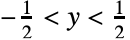
Plot[{Exp[x], Log[x], x}, {x, -3, 3}, PlotRange -> 3, PlotStyle -> {Red, Green, Dashed}, AspectRatio -> Automatic]区間内で-Abs[x]≤x Sin[1/x]≤Abs[x]であることを示す:
Plot[{x Sin[1 / x], Abs[x], -Abs[x]}, {x, -1 / 2, 1 / 2}, PlotStyle -> {Red, Directive[Dashed, Gray], Directive[Dashed, Gray]}]離散関数の特性のハイライト (8)
Plot[Tan[x], {x, -5, 5}]ExclusionsStyleを指定して特異値を強調する:
Plot[Tan[x], {x, -5, 5}, ExclusionsStyle -> Dashed]ExclusionsStyleを使って関数  における不連続性をハイライトする:
Plot[Sin[Floor[x]], {x, 0, 10}, ExclusionsStyle -> Dotted]Plot[Sin[Floor[x]], {x, 0, 10}, Exclusions -> {Sin[π x] == 0}, ExclusionsStyle -> Dashed]
Plot[Sin[Sqrt[2]x] + Sin[x], {x, 0, 20}]MeshFunctionsに渡される第2引数は  である:
Plot[Sin[Sqrt[2]x] + Sin[x], {x, 0, 20}, MeshFunctions -> {Function[{x, y}, y]}, Mesh -> {{0}}, MeshStyle -> Directive[PointSize[Medium], Red]]MeshFunctionsを使って関数  の極値をハイライトする:
Plot[Sin[Sqrt[2]x] + Sin[x], {x, 0, 50}]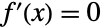
mf = Function[{x, y}, Evaluate@D[Sin[Sqrt[2]x] + Sin[x], x]];Plot[Sin[Sqrt[2]x] + Sin[x], {x, 0, 50}, MeshFunctions -> {mf}, Mesh -> {{0}}, MeshStyle -> Directive[PointSize[Medium], Red]]
f = Sin[Sqrt[2]x] + Sin[x];Plot[f, {x, 0, 50}]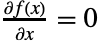
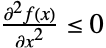
Plot[f, {x, 0, 50}, Exclusions -> {{D[f, x] == 0, D[f, {x, 2}] ≤ 0}}, ExclusionsStyle -> Directive[Thickness[0.02], Red]]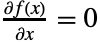
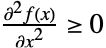
Plot[f, {x, 0, 50}, Exclusions -> {{D[f, x] == 0, D[f, {x, 2}] ≥ 0}}, ExclusionsStyle -> Directive[Thickness[0.02], Purple]]
f = Sin[Sqrt[2]x] + Sin[x];Plot[f, {x, 0, 50}]Filling指定を使うと上記が容易に達成できる:
Plot[f, {x, 0, 50}, Filling -> {{1 -> {0, {Red, Blue}}}}, PlotLegends -> SwatchLegend[{Blue, Red}, {"non-negative", "non-positive"}]]
f = Sin[Sqrt[2]x] + Sin[x];plot = Plot[f, {x, 0, 50}]
rfi = Function[{x, y}, Evaluate[D[f, x] ≥ 0]];incr = Plot[f, {x, 0, 50}, RegionFunction -> rfi, PlotStyle -> Blue]
rfd = Function[{x, y}, Evaluate[D[f, x] ≤ 0]];decr = Plot[f, {x, 0, 50}, RegionFunction -> rfd, PlotStyle -> Red]Legended[Show[incr, decr], SwatchLegend[{Blue, Red}, {"increasing", "decreasing"}]]
f = Sin[Sqrt[2]x] + Sin[x];plot = Plot[f, {x, 0, 50}]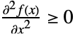
rfcvx = Function[{x, y}, Evaluate[D[f, {x, 2}] ≥ 0]];cvx = Plot[f, {x, 0, 50}, RegionFunction -> rfcvx, PlotStyle -> Orange]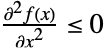
rfccv = Function[{x, y}, Evaluate[D[f, {x, 2}] ≤ 0]];ccv = Plot[f, {x, 0, 50}, RegionFunction -> rfccv, PlotStyle -> Blue]Legended[Show[cvx, ccv], SwatchLegend[{Orange, Blue}, {"convex", "concave"}]]連続関数の特性のハイライト (1)


f = Sin[Sqrt[2]x] + Sin[x];Plot[f, {x, 0, 20}]0から1の間になるように導関数を再スケールすると,簡単に色にマップできる:
{min, max} = {NMinValue[{D[f, x], 0 ≤ x ≤ 20}, x], NMaxValue[{D[f, x], 0 ≤ x ≤ 20}, x]};df = Rescale[D[f, x], {min, max}, {0, 1}]Plot[df, {x, 0, 20}]ColorDataからさまざまなカラースケールが得られる:
cf = Function[{x}, Evaluate[ColorData["Rainbow"][ df]]]leg = BarLegend[{ColorData["Rainbow"][Rescale[#, {min, max}, {0, 1}]]&, {min, max}}, LegendMarkerSize -> 150];ColorFunctionを使って曲線の上に色として導関数が重ねられた:
Plot[f, {x, 0, 20}, ColorFunction -> cf, ColorFunctionScaling -> False, PlotLegends -> leg]Fillingを使うと色がさらに強調される:
Plot[f, {x, 0, 20}, ColorFunction -> cf, ColorFunctionScaling -> False, Filling -> 0, PlotLegends -> leg]関数のエピグラフとハイポグラフ (2)




複素数値の関数 (3)
Plot[{Re[Exp[I ω]], Im[Exp[I ω]]}, {ω, 0, 10}, PlotLegends -> "Expressions"]Plot[{Abs[Exp[I ω] / (1 + ω^2)], Arg[Exp[I ω] / (1 + ω^2)]}, {ω, -π, π}, PlotLegends -> "Expressions"]f = Exp[I ω] / (1 + ω^2);
cf = Function[ω, Evaluate[Hue[Arg[f] / (2π), 0.5]]]Plot[Abs[f], {ω, -π, π}, ColorFunction -> cf, ColorFunctionScaling -> False]Plot[Abs[f], {ω, -π, π}, ColorFunction -> cf, ColorFunctionScaling -> False, Filling -> Bottom, PlotLegends -> BarLegend[{cf, {-π, π}}, LegendMarkerSize -> 150]]方程式の解法 (2)
s = DSolve[y'[x] == (1/1 + y[x]), y, x]Plot[Evaluate[y[x] /. s /. C[1] -> 0], {x, -2, 5}]Plot[Evaluate[y[x] /. s /. C[1] -> Range[0, 5]], {x, -5, 5}]s = Reduce[Sin[x ^ 2 + y] == 0, {x, y}]Plot[Evaluate[{-x^2 + 2 π C[1], π - x^2 + 2 π C[1]} /. C[1] -> Range[-5, 5]], {x, -5, 5}]特性と関係 (9)
Plotは必要であればより多くの点を使う:
Plot[Sin[x], {x, 0, 10}, Mesh -> All]Plotは曲線におけるParametricPlotの特殊ケースである:
{Plot[Sin[x ^ 2], {x, 0, 5}], ParametricPlot[{x, Sin[x ^ 2]}, {x, 0, 5}, AspectRatio -> 1 / GoldenRatio]}パラメトリック曲線と領域にParametricPlotを使う:
{ParametricPlot[{Cos[θ], Sin[θ]}, {θ, 0, 2Pi}], ParametricPlot[{r Cos[θ], r Sin[θ]}, {θ, 0, 2Pi}, {r, 1, 2}]}陰的な曲線と領域にContourPlotとRegionPlotを使う:
{ContourPlot[x ^ 2 + y ^ 2 == 1, {x, -1, 1}, {y, -1, 1}], RegionPlot[1 < x ^ 2 + y ^ 2 < 4, {x, -2, 2}, {y, -2, 2}]}対数プロットにLogPlot,LogLinearPlot,LogLogPlotを使う:
LogLogPlot[Abs[10 ^ 2 / ((I ω) ^ 2 + 100)], {ω, 10 ^ 0, 10 ^ 5}]データにListPlotとListLinePlotを使う:
{ListLinePlot[Table[{x, Sin[x]}, {x, 0, 10, 0.25}]], Plot[Sin[x], {x, 0, 10}]}AbsArgPlotは,Plotの特殊ケースである:
{Plot[Abs[ArcSin[x]], {x, -3, 3}],
AbsArgPlot[ArcSin[x], {x, -3, 3}]}{Plot[ReIm[ArcSin[x]], {x, -3, 3}],
ReImPlot[ArcSin[x], {x, -3, 3}]}関数とパラメータ的な曲面にPlot3DとParametricPlot3Dを使う:
Plot3D[(x ^ 2 + y ^ 2)Exp[-(x ^ 2 + y ^ 2)], {x, -2, 2}, {y, -2, 2}]ParametricPlot3D[{-2 Cos[u] Cos[v] ^ 3, -2 Cos[v] ^ 2 Sin[u], 2 Tan[v]}, {u, 0, 2Pi}, {v, -1, 1}]関連リンク

 プログラミングの基本:グラフィックス
テキスト
Wolfram Research (1988), Plot, Wolfram言語関数, https://reference.wolfram.com/language/ref/Plot.html (2026年に更新).
CMS
Wolfram Language. 1988. "Plot." Wolfram Language & System Documentation Center. Wolfram Research. Last Modified 2026. https://reference.wolfram.com/language/ref/Plot.html.
APA
Wolfram Language. (1988). Plot. Wolfram Language & System Documentation Center. Retrieved from https://reference.wolfram.com/language/ref/Plot.html