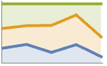
 曲線は




StackedListPlot
StackedListPlot[{data1,data2,…}]
各 dataiの線をプロットする.第 i 曲線は data1から dataiまでの値の累積になる.
StackedListPlot[{…,w[datai],…}]
記号ラッパー w によって定義された特徴とともに dataiをプロットする.
詳細とオプション
- dataiには次の形式と解釈がある.
-
{y1,y2,…} 高さ{y1,y2,…}と自動的に決定される x の値 {{x1,y1},{x2,y2},…} 値{{x1,y1},{x2,y2},…} <"k1"y1,"k2"y2,…> 値{y1,y2,…} <x1y1,x2y2,…> キーと値のペア{{x1,y1},{x2,y2},…} {y1"lbl1",y2"lbl2",…}, {y1,y2,…}{"lbl1","lbl2",…} ラベル{lbl1,lbl2,…}が付いた値{y1,y2,…} SparseArray 正規配列としての値 TimeSeries, EventSeries 時間と値のペア QuantityArray 大きさ WeightedData 重みなしの値 - データ値 xiおよび yiは次の形で与えることができる.
-
xi 実数値の数 Quantity[xi,unit] 単位が付いた数量 Around[xi,ei] 不確かさが eiの値 xi Interval[{xmin,xmax}] xminから xmaxまでの値 - 必要であれば,データは xiに従ってソートされる.
- dataiの正の部分は正の軸上に,負の部分は負の軸上にプロットされる,
- yiの負の値は正の値とは反対の方向に積み重ねられる.
- 上記以外の形式の xiと yiの値は欠落値とみなされ,表示されない.欠落データは累積の際には0とみなされる.
- StackedListPlot[Tabular[…]cspec]は,列指定 cspec を使って表オブジェクトから値を抽出し,これをプロットする.
- 次は,表形式データのプロットに使用可能な列指定 cspec の形式である.
-
{colx,coly} 列 y と列 x をプロットする {{colx1,coly1},{colx2,coly2},…} 列 y1と列 x1,列 y2と列 x2をプロットする等 coly, {coly} 列 y を一連の値としてプロットする {{coly1},…,{colyi},…} 列 y1, y2, …を一連の値としてプロットする - StackedListPlot[TimeSeries[…]{com1,com2,…}]およびStackedListPlot[EventSeries[…]{com1,com2,…}]は,時系列または事象系列の成分{col1,col2,…}を抽出し,タイムスタンプに対してプロットする.
- colxはAutomaticでもよい.その場合は,DataRangeを使って一連の値が生成される.
- dataiには次のラッパー w を使うことができる.
-
Annotation[datai,label] データについての注釈を与える Button[datai,action] データがクリックされた際に実行するアクションを定義する Callout[datai,label] コールアウトでデータにラベルを付ける Callout[datai,label,pos] 相対位置 pos にコールアウトを置く EventHandler[datai,events] データの一般的なイベントハンドラを定義する Highlighted[datai,effect] 効果を使って fiを動的にハイライトする Highlighted[datai,Placed[effect,pos]] 位置 pos で効果を使って fiを静的にハイライトする Hyperlink[datai,uri] データをハイパーリンクにする Labeled[datai,label] データにラベルを付ける Labeled[datai,label,pos] ラベルを相対位置 pos に置く Legended[datai,label] データを凡例で識別する PopupWindow[datai,cont] データにポップアップウィンドウを付ける StatusArea[datai,label] マウスが上に置かれたときにステータスエリアに表示する Style[datai,styles] 指定したスタイルを使ってデータを示す Tooltip[datai,label] 曲線にツールチップを付ける - ラッパー w は複数のレベルで適用することができる.
-
{…,w[yi],…} データの値 yiを囲む {…,w[{xi,yi}],…} 点{xi,yi}を囲む w[datai] データを囲む w[{data1,…}] dataiの集合を囲む w1[w2[…]] ネストしたラッパーを使う - Callout,LabeledとPlacedには次の位置 pos が使える.
-
Automatic 自動的に置かれたラベル Above, Below, Before, After 曲線の周りの位置 x 位置 x の曲線の近く Scaled[s] 曲線に沿ってスケールされた位置 s {s,Above},{s,Below},… 曲線に沿った位置 s の相対的な位置 {pos,epos} 曲線と相対的な位置 pos に置かれたラベル中の epos - StackedListPlotには,Graphicsと同じオプションに以下の追加・修正を加えたものが使われる. [全オプションのリスト]
- DataRangeは,値{y1,…,yn}をどのように{{x1,y1},…,{xn,yn}}と解釈するかを決定する.次は使用可能な設定である.
-
Automatic,All 1から n まで一様に {xmin,xmax} xminから xmaxまで一様に - 一般に,ペアのリスト{{x1,y1},{x2,y2},…}は点のリストとして解釈されるが,DataRangeAllという設定はそれを複数のデータソース{{y11,y12},{y21,y23},…}として解釈するように強制する.
- LabelingFunction->f は,各点に f[value,index,lbls]で与えられたラベルを付けるように指定する.ただし,value は点に関連付けた値,index は data 内の位置,lbls は関係するラベルのリストである.
- 次は,データの複数の集合を表示する際に使えるPlotLayoutの設定である.
-
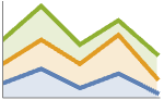
"Stacked" 軸ごとにデータを積み重ねる 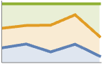
"Percentile" 軸ごとにデータを積み重ねて正規化する - PlotLegendsのよく使われる設定値
-
None 凡例は付けない Automatic 凡例を自動的に決定する {lbl1,lbl2,…} 凡例のラベルとして lbl1, lbl2, …を使う Placed[lspec,…] 凡例の置き方を指定する - PlotStylesty は,各曲線のスタイルを指定する.使用可能な設定には以下がある.
-
{sty1,sty2,…} データ集合の一連のスタイル <"key"val,…> 異なるレベルのデータについてのスタイル要素 - 使用可能なキーには以下がある.
-
"Base" dataiすべての全体的なスタイル "Lists" 各 dataiについてのスタイル styiのリスト - ColorData["DefaultPlotColors"]は,PlotStyleで使われるデフォルトの色のシーケンスを与える.
- ScalingFunctions->"scale"が
 座標をスケールする.ScalingFunctions{"scalex","scaley"}は
 座標と
 座標の両方をスケールする.
- 次は,HighlightedとPlotHighlightingに使用可能なハイライト効果である.
-
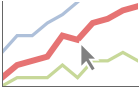
style 指定された曲線をハイライトする 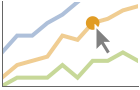
"Ball" 曲線上の指定された点をハイライトしてラベルを付ける 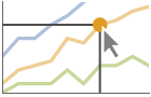
"Dropline" 曲線上の指定された点を軸までのドロップラインでハイライトしてラベルを付ける 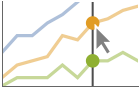
"XSlice" 垂直スライスに沿ったすべての点をハイライトしてラベルを付ける 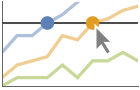
"YSlice" 水平スライスに沿ったすべての点をハイライトしてラベルを付ける 
Placed[effect,pos] 指定の位置 pos を静的にハイライトする - ハイライトの位置指定 pos には次がある.
-
{x} {x,y}における効果.y は自動的に選択される {x,y} {x,y}における効果 {pos1,pos2,…} 複数の位置 posi
全オプションのリスト
例題
すべて開く すべて閉じる例 (4)

StackedListPlot[{{3, 2, 1, 6, 4, 7, 7, 2, 3, 1}, {7, 8, 8, 3, 5, 9, 10, 3, 10, 10}, {10, 2, 4, 8, 4, 10, 8, 4, 5, 3}}]

d = {{{16, 78}, {25, 51}, {44, 87}, {64, 62}, {87, 16}, {93, 19}}, {{14, 34}, {41, 75}, {59, 80}, {61, 90}, {67, 19}, {79, 22}}, {{24, 93}, {36, 80}, {53, 53}, {93, 98}, {99, 55}, {100, 54}}};StackedListPlot[d]StackedListPlot[MapIndexed[Callout[#, IntegerName[First[#2], "Ordinal"]]&, RandomInteger[{1, 10}, {3, 10}]], ImageSize -> 300]StackedListPlot[Quantity[RandomInteger[{1, 10}, {3, 10}], "Centimeters"], AxesLabel -> Automatic]スコープ (30)
一般的なデータ (5)
d = {{{6.7, 5.4}, {7.8, 8.1}, {8.1, 7.0}, {8.9, 7.3}, {10., 9.}}, {{5.4, 5.9}, {7.8, 5.6}, {8., 7.8}, {8.5, 5.2}, {8.6, 7.}}, {{6.2, 8.4}, {6.3, 5.8}, {6.4, 9.9}, {6.5, 5.2}, {8.1, 8.0}}};StackedListPlot[d, PlotMarkers -> Automatic]StackedListPlot[{{1, 2, 4, 2, 5, 1}, {1, 1, 1, Missing[], 1, 1}, {1, 2, 3, 4, 5, 6}}]data = {{1, -2, 3, 4, 5}, {1, 2, -3, 4, 5}, {1, 2, 3, -4, 5}};StackedListPlot[data]d = RandomInteger[{1, 10}, {3, 10}];StackedListPlot[d, PlotLayout -> "Percentile"]ScalingFunctionsを使って軸をスケールする:
d = RandomInteger[{1, 1000}, {3, 10}];StackedListPlot[d, ScalingFunctions -> "Log"]表形式データ (1)
tab = Tabular[IconizedObject[«Country populations»]]フランス,イギリス,日本の1940年から2020年までの総人口をプロットする:
StackedListPlot[tab -> {{"Date", "France"}, {"Date", "UK"}, {"Date", "Japan"}}]StackedListPlot[tab -> {{"Date", "France"}, {"Date", "UK"}, {"Date", "Japan"}}, PlotLayout -> "Percentile"]StackedListPlot[tab -> {{"Date", "France"}, {"Date", "Germany"}, {"Date", "Australia"}}, PlotLegends -> {"France", "UK", "Japan"}]特殊なデータ (5)
Quantityを使ってデータに単位を付ける:
d = RandomInteger[{1, 10}, {3, 10}];StackedListPlot[Quantity[d, "Meters"], AxesLabel -> Automatic]d = {1, 4, 2, 3, 10, 8, 2};StackedListPlot[{d -> {"a", "b", "c", "d", "e", "f", "g"}, d}]StackedListPlot[{d, {2, 3, 5, 7, 11, 13, 17} -> {"a", "b", "c", "d", "e", "f", "g"}}]d = {1, 4, 2, 3, 10, 8, 2};StackedListPlot[{d, {2, 3, 5, 7, 11, 13, 17} -> {"a", "b", "c", "d", "e", "f", "g"}}, LabelingFunction -> Above]TimeSeriesを直接プロットする:
data = {CountryData["UnitedStates", {{"Population"}, {1988, 2013}}], CountryData["China", {{"Population"}, {1988, 2013}}]};StackedListPlot[data, AxesLabel -> Automatic, PlotLabels -> {"USA", "China"}]StackedListPlot[Table[Around[RandomInteger[{1, 25}], RandomReal[5]], 3, 10]]StackedListPlot[Table[Interval[RandomInteger[25, 2]], 3, 10]]StackedListPlot[Table[Around[RandomInteger[{1, 25}], RandomReal[5]], 3, 10], IntervalMarkers -> "Bands"]データのラッパー (3)
{StackedListPlot[{Style[{1, 2, 3}, Green], {4, 5, 6}}], StackedListPlot[Style[{{1, 2, 3}, {4, 5, 6}}, Blue]]}d = {1, 4, 2, 3, 10, 8, 2};StackedListPlot[{d, Tooltip@d}, Mesh -> Full]StackedListPlot[{d, Tooltip[d, "Second"]}]PopupWindowを使って追加的なドリルダウン情報を与える:
d = {1, 4, 2, 3, 10, 8, 2};StackedListPlot[{d, PopupWindow[{1, 2, 3}, Graphics[Circle[]]]}]Buttonを使って任意のアクションを起こすことができる:
StackedListPlot[{d, Button[{1, 2, 3}, Speak["Hello"]]}]ラベルと凡例 (10)
Labeledでデータソースにラベルを付ける:
data = RandomInteger[{1, 25}, {3, 10}];StackedListPlot[MapThread[Labeled[#1, #2]&, {data, {"First", "Second", "Third"}}]]PlotLabelsでラベルを指定する:
data = RandomInteger[{1, 25}, {3, 10}];StackedListPlot[data, PlotLabels -> {"First", "Second", "Third"}]Calloutでデータに自動的にラベルを付ける:
data = RandomInteger[{1, 25}, {3, 10}];StackedListPlot[{Callout[data[[1]], "First"], Callout[data[[2]], "Second"], Callout[data[[3]], "Third"]}]StackedListPlot[data, PlotLegends -> {"First", "Second", "Third"}]data = Table[Labeled[Prime[i], RandomWord[]], {i, 10}];StackedListPlot[{data, data}, LabelingSize -> 30]StackedListPlot[{data, data}, LabelingSize -> Full]密な点集合については,デフォルトで,ラベルの一部がツールチップに変換されることもある:
data = Sort[Table[Callout[RandomReal[1, 2], i], {i, 150}]];StackedListPlot[{data, data}]プロットサイズを大きくすると,表示されるラベル数も多くなる:
StackedListPlot[{data, data}, ImageSize -> 400]Legendedを使って特定のデータ集合に凡例を付ける:
upper = RandomReal[{1.5, 2}, 50];
lower = RandomReal[0.5, 50];StackedListPlot[{lower, Legended[Mean[{lower, upper}], "average"], upper}]Placedを使って凡例の位置を変える:
StackedListPlot[{lower, Legended[Mean[{lower, upper}], Placed["average", Below]], upper}]StackedListPlot[<|"fibonacci" -> Fibonacci[Range[10]], "stacked primes" -> Prime[Range[10]]|>, PlotLabels -> Automatic, PlotLegends -> None]プロットには,通常,マウスオーバーの際に座標を示すインタラクティブなコールアウトが付いている:
StackedListPlot[{{...}, {...}}]特定のラッパーあるいはツールチップのようなインタラクションを含めることでインタラクティブ機能をオフにする:
StackedListPlot[Callout[{...}, "hello", 13]]{StackedListPlot[{{...}, {...}}, PlotHighlighting -> "Dropline"], StackedListPlot[{{...}, {...}}, PlotHighlighting -> "XSlice"]}Highlightedを使ってプロット上の特定の点を強調する:
StackedListPlot[Highlighted[{{...}, {...}}, Placed["Ball", 7]]]StackedListPlot[Highlighted[{{...}, {...}}, Placed["Ball", {{6}, {15}}]]]プレゼンテーション (6)
data = RandomInteger[{1, 25}, {3, 5, 2}];StackedListPlot[data]StackedListPlot[data, PlotStyle -> {Dashed, Red, Green}, PlotMarkers -> True]StackedListPlot[data, PlotTheme -> "Marketing"]data = {{23, 17, 22, 8, 4, 14, 6, 18, 18, 3}, {9, 16, 2, 24, 2, 12, 5, 25, 11, 4}};StackedListPlot[data, AxesLabel -> {k, None}, PlotLabel -> "Stacked data"]data1 = {23, 17, 22, 8, 4, 14, 6, 18, 18, 3};
data2 = {9, 16, 2, 24, 2, 12, 5, 25, 11, 4};StackedListPlot[{Tooltip[data1, "first"], Tooltip[data2, "second"]}]StackedListPlot[RandomInteger[{1, 25}, {2, 10}], Filling -> {1 -> {2}}]StackedListPlot[RandomInteger[{1, 25}, {3, 5, 2}], Mesh -> 10]StackedListPlot[RandomInteger[{1, 25}, {3, 5, 2}], Mesh -> 10, MeshShading -> {Red, None, Blue}]オプション (95)
AspectRatio (4)
デフォルトで,StackedListPlotはプロットに固定の縦横比を使う:
StackedListPlot[RandomInteger[{1, 10}, {3, 10}]]AspectRatio1として高さと幅を等しくする:
StackedListPlot[RandomInteger[{1, 10}, {3, 10}], AspectRatio -> 1]AspectRatioAutomaticとするプロット範囲から縦横比が決められる:
StackedListPlot[RandomInteger[{1, 10}, {3, 10}], AspectRatio -> Automatic]AspectRatioFullとすると,他の構造物内にぴったり納まるように高さと幅が調整される:
plot = StackedListPlot[RandomInteger[{1, 10}, {3, 10}], AspectRatio -> Full];
{Framed[Pane[plot, {50, 100}]], Framed[Pane[plot, {100, 100}]], Framed[Pane[plot, {100, 50}]]}
Axes (3)
StackedListPlot[RandomInteger[{1, 10}, {3, 10}]]StackedListPlot[RandomInteger[{1, 10}, {3, 10}], Axes -> False]{StackedListPlot[RandomInteger[{1, 10}, {3, 10}], Axes -> {True, False}], StackedListPlot[RandomInteger[{1, 10}, {3, 10}], Axes -> {False, True}]}AxesLabel (4)
StackedListPlot[RandomInteger[{1, 10}, {3, 10}], Frame -> False, Axes -> True]
StackedListPlot[RandomInteger[{1, 10}, {3, 10}], Frame -> False, Axes -> True, AxesLabel -> value]StackedListPlot[RandomInteger[{1, 10}, {3, 10}], Frame -> False, Axes -> True, AxesLabel -> {position, value}]StackedListPlot[QuantityArray[RandomInteger[{1, 10}, {3, 10}], "Meters"], Frame -> False, Axes -> True, AxesLabel -> Automatic]AxesOrigin (2)
AxesStyle (4)
StackedListPlot[RandomInteger[{1, 10}, {3, 10}], AxesStyle -> Red]StackedListPlot[RandomInteger[{1, 10}, {3, 10}], AxesStyle -> {{Thick, Red}, {Thick, Blue}}]StackedListPlot[RandomInteger[{1, 10}, {3, 10}], AxesStyle -> Green, TicksStyle -> Red]StackedListPlot[RandomInteger[{1, 10}, {3, 10}], AxesStyle -> Green, LabelStyle -> Red]ClippingStyle (1)
d = Table[Sin[x], {x, -3, 3}];StackedListPlot[{d, d}, PlotRange -> {-.7, .7}, ClippingStyle -> {Red, Green}]StackedListPlot[{d, d}, ClippingStyle -> Automatic, PlotRange -> {-.7, .7}, PlotStyle -> Thick]StackedListPlot[{d, d}, PlotRange -> {-.7, .7}, ClippingStyle -> Red]StackedListPlot[{d, d}, PlotRange -> {-.7, .7}, ClippingStyle -> {Red, Thick}]StackedListPlot[{d, d}, PlotRange -> {-.7, .7}, ClippingStyle -> Directive[Red, Thick]]DataRange (4)
StackedListPlot[RandomInteger[{1, 10}, {3, 10}]]StackedListPlot[RandomInteger[{1, 10}, {3, 10}], DataRange -> {0, 2}]StackedListPlot[RandomInteger[{1, 10}, {3, 10}], DataRange -> {0, 1}]

d = Transpose[{Range[10], #}]& /@ RandomInteger[{1, 10}, {3, 10}];StackedListPlot[d] 値がデータの一部であるので,DataRangeを指定してもこの場合は影響が出ない:
StackedListPlot[d, DataRange -> {0, 1}]StackedListPlot[{{1, 1}, {2, 2}, {3, 2}}, DataRange -> All, AxesOrigin -> {1, 0}]Filling (3)
d = RandomInteger[{1, 10}, {3, 10}];Table[StackedListPlot[d, Filling -> c], {c, {Top, Bottom, Axis, Prime[15]}}]StackedListPlot[RandomInteger[{1, 10}, {3, 10}], Filling -> Axis]StackedListPlot[RandomInteger[{1, 10}, {3, 10}], Filling -> {1 -> Axis}]StackedListPlot[RandomInteger[{1, 10}, {3, 10}], Filling -> {1 -> {2}}]StackedListPlot[RandomInteger[{1, 10}, {3, 10}], Filling -> {1 -> {{2}, Hue[.6]}}]
StackedListPlot[RandomInteger[{1, 10}, {3, 10}], Filling -> {1 -> {1 / 2, LightOrange}}]FillingStyle (2)
d = RandomInteger[{1, 10}, {2, 10}];Table[StackedListPlot[d, Filling -> Axis, FillingStyle -> c], {c, {Red, Green, Blue, Yellow}}]StackedListPlot[RandomInteger[{1, 10}, {3, 10}], Filling -> Axis, FillingStyle -> Directive[Opacity[0.5], Orange]]StackedListPlot[RandomInteger[{-10, 10}, {3, 10}], Filling -> Axis, FillingStyle -> {Red, Blue}]ColorFunctionから得た変化する色での塗潰しスタイルを使う:
StackedListPlot[RandomInteger[{1, 10}, {3, 10}], ColorFunction -> Function[{x, y}, Hue[y]], Filling -> Axis, FillingStyle -> Automatic]ImageSize (7)
Tiny,Small,Medium,Largeのような名前付きのサイズを使う:
{StackedListPlot[RandomInteger[{1, 10}, {3, 10}], ImageSize -> Tiny], StackedListPlot[RandomInteger[{1, 10}, {3, 10}], ImageSize -> Small]}{StackedListPlot[RandomInteger[{1, 10}, {3, 10}], ImageSize -> 150], StackedListPlot[RandomInteger[{1, 10}, {3, 10}], AspectRatio -> 1.5, ImageSize -> 150]}{StackedListPlot[RandomInteger[{1, 10}, {3, 10}], ImageSize -> {Automatic, 150}], StackedListPlot[RandomInteger[{1, 10}, {3, 10}], AspectRatio -> 2, ImageSize -> {Automatic, 150}]}{StackedListPlot[RandomInteger[{1, 10}, {3, 10}], ImageSize -> UpTo[200]], StackedListPlot[RandomInteger[{1, 10}, {3, 10}], AspectRatio -> 2, ImageSize -> UpTo[200]]}グラフィックスの幅と高さを指定して,必要な場合はスペースで充填する:
StackedListPlot[RandomInteger[{1, 10}, {3, 10}], ImageSize -> {200, 300}, Background -> StandardBrown]AspectRatioFullと設定すると,使用可能なスペースが塗り潰される:
StackedListPlot[RandomInteger[{1, 10}, {3, 10}], AspectRatio -> Full, ImageSize -> {200, 300}, Background -> StandardBrown]{StackedListPlot[RandomInteger[{1, 10}, {3, 10}], ImageSize -> {UpTo[150], UpTo[100]}], StackedListPlot[RandomInteger[{1, 10}, {3, 10}], AspectRatio -> 2, ImageSize -> {UpTo[150], UpTo[100]}]}ImageSizeFullを使ってオブジェクト内の使用可能なスペースを塗り潰す:
Framed[Pane[StackedListPlot[RandomInteger[{1, 10}, {3, 10}], ImageSize -> Full, Background -> StandardBrown], {200, 100}]]Framed[Pane[StackedListPlot[RandomInteger[{1, 10}, {3, 10}], AspectRatio -> Full, ImageSize -> {Scaled[0.5], Scaled[0.5]}, Background -> StandardBrown], {200, 200}]]InterpolationOrder (1)
StackedListPlot[RandomInteger[{1, 10}, {3, 10}], Mesh -> Full]StackedListPlot[RandomInteger[{1, 10}, {3, 10}], InterpolationOrder -> 2, Mesh -> Full]StackedListPlot[RandomInteger[{1, 10}, {3, 10}], InterpolationOrder -> 0, Mesh -> Full]IntervalMarkers (3)
StackedListPlot[Table[Around[RandomInteger[{1, 25}], RandomReal[3]], 3, 10]]StackedListPlot[Table[Around[RandomInteger[{1, 25}], RandomReal[3]], 3, 10], IntervalMarkers -> "Bars"]StackedListPlot[Table[Around[RandomInteger[{1, 25}], RandomReal[3]], 3, 10], IntervalMarkers -> "Bands"]IntervalMarkersStyle (2)
LabelingFunction (1)
d = {1, 4, 2, 3, 10, 8, 2};StackedListPlot[{d -> {"a", "b", "c", "d", "e", "f", "g"}, d}]LabelingFunction->Noneを使ってラベルが付かないようにする:
StackedListPlot[{d -> {"a", "b", "c", "d", "e", "f", "g"}, d}, LabelingFunction -> None]StackedListPlot[{d -> {"a", "b", "c", "d", "e", "f", "g"}, d}, LabelingFunction -> Above]StackedListPlot[{d -> {"a", "b", "c", "d", "e", "f"}, d}, LabelingFunction -> Callout[Automatic, Automatic]]StackedListPlot[{d -> {"a", "b", "c", "d", "e", "f", "g"}, d}, LabelingFunction -> (#1&)]StackedListPlot[{d -> {"a", "b", "c", "d", "e", "f", "g"}, d}, LabelingFunction -> (#2&)]LabelingSize (4)
data = {1, 1, 2, 3, 5, 8} -> {"healthfulness", "obstreperous", "spectrogram", "vestige", "coinage", "limey"};StackedListPlot[{data, data}, ImageSize -> Medium]data = {1, 1, 2, 3, 5, 8} -> {[image], [image], [image], [image], [image], [image]};StackedListPlot[{data, data}, ImageSize -> Medium]data = {1, 1, 2, 3, 5, 8} -> {"healthfulness", "obstreperous", "spectrogram", "vestige", "coinage", "limey"};StackedListPlot[{data, data}, ImageSize -> Medium, LabelingSize -> 30]data = {1, 1, 2, 3, 5, 8} -> {[image], [image], [image], [image], [image], [image]};StackedListPlot[{data, data}, ImageSize -> Medium, LabelingSize -> 20]data = {1, 1, 2, 3, 5, 8} -> {[image], [image], [image], [image], [image], [image]};StackedListPlot[{data, data}, ImageSize -> Medium, LabelingSize -> Full]LabelingTarget (6)
StackedListPlot[{IconizedObject[«Subscript[data, 1]»], IconizedObject[«Subscript[data, 2]»]}]StackedListPlot[{IconizedObject[«Subscript[data, 1]»], IconizedObject[«Subscript[data, 2]»]}, LabelingTarget -> All]StackedListPlot[{IconizedObject[«Subscript[data, 1]»], IconizedObject[«Subscript[data, 2]»]}, LabelingTarget -> "Dense"]StackedListPlot[{IconizedObject[«Subscript[data, 1]»], IconizedObject[«Subscript[data, 2]»]}, LabelingTarget -> 0.5]StackedListPlot[{IconizedObject[«Subscript[data, 1]»], IconizedObject[«Subscript[data, 2]»]}, LabelingTarget -> <|"AllowedLabelingPositions" -> "Sides"|>]StackedListPlot[{IconizedObject[«Subscript[data, 1]»], IconizedObject[«Subscript[data, 2]»]}, LabelingTarget -> <|"AllowedLabelingPositions" -> "Corners"|>]StackedListPlot[{IconizedObject[«Subscript[data, 1]»], IconizedObject[«Subscript[data, 2]»]}, LabelingTarget -> <|"AllowLabelClipping" -> True|>]MaxPlotPoints (1)
Mesh (1)
d = RandomInteger[{1, 10}, {3, 10}];{StackedListPlot[d, Mesh -> Full], StackedListPlot[d, Mesh -> All]}{StackedListPlot[d, Mesh -> Full, InterpolationOrder -> 2], StackedListPlot[d, Mesh -> All, InterpolationOrder -> 2]}
StackedListPlot[d, Mesh -> 20]
StackedListPlot[d, Mesh -> {Range[0, 2Pi, Pi / 4]}, MeshStyle -> PointSize[Medium]]
StackedListPlot[d, Mesh -> {Table[{x, Hue[x / (2Pi)]}, {x, 0., 2Pi, 2Pi / 8}]}]MeshFunctions (1)


d = RandomInteger[{1, 10}, {3, 10}];Table[StackedListPlot[d, MeshFunctions -> {Function[{x, y}, Evaluate[f]]}, Mesh -> 9, PlotLabel -> f], {f, {x, y}}] 方向(赤)に3つのメッシュレベルを,
 方向(青)に10のメッシュレベルを使う:
StackedListPlot[d, Mesh -> {3, 10}, MeshFunctions -> {#1&, #2&}, MeshStyle -> {Directive[PointSize[Medium], Red], Blue}]MeshShading (1)

d = RandomInteger[{1, 10}, {3, 10}];StackedListPlot[d, Mesh -> 10, MeshFunctions -> {#1&}, MeshShading -> {Red, Blue}]Noneを使って線分を削除する:
StackedListPlot[d, Mesh -> 10, MeshFunctions -> {#1&}, MeshShading -> {Red, None}]MeshShadingはPlotStyleとともに使うことができる:
StackedListPlot[d, Mesh -> 10, PlotStyle -> Thick, MeshFunctions -> {#1&}, MeshShading -> {Red, Blue}]曲線のスタイル付けでは,MeshShadingはPlotStyleより優先順位が高い:
StackedListPlot[d, Mesh -> 10, PlotStyle -> StandardGray, MeshFunctions -> {#1&}, MeshShading -> {Red, Blue}]MeshShadingをAutomaticに設定し,いくつかの線分にPlotStyleを使う:
StackedListPlot[d, Mesh -> 10, PlotStyle -> Directive[Thick, Yellow], MeshFunctions -> {#1&}, MeshShading -> {Red, Automatic}]MeshShadingはColorFunctionとともに使うことができる:
StackedListPlot[d, Mesh -> 10, PlotStyle -> Thick, MeshFunctions -> {#1&}, MeshShading -> {Black, Automatic},
	ColorFunction -> Function[{x, y}, Hue[x]]]
MeshStyle (1)
d = RandomInteger[{1, 10}, {3, 10}];StackedListPlot[d, Mesh -> 10, MeshStyle -> Automatic]
StackedListPlot[d, Mesh -> 10, MeshStyle -> Red]

StackedListPlot[d, Mesh -> 10, MeshStyle -> {Red, Blue}, MeshFunctions -> {#1&, #2&}]
StackedListPlot[d, Mesh -> 10, MeshStyle -> Directive[PointSize[Large], Red]]PlotHighlighting (7)
デフォルト設定のPlotHighlightingAutomaticのとき,プロットにはインタラクティブな座標のコールアウトが付く:
StackedListPlot[{IconizedObject[«primes»], IconizedObject[«squares»]}]PlotHighlightingNoneを使ってプロット全体のハイライトをオフにする:
StackedListPlot[{IconizedObject[«primes»], IconizedObject[«squares»]}, PlotHighlighting -> None]Highlighted[…,None]を使って単一の集合のハイライトをオフにする:
StackedListPlot[{IconizedObject[«primes»], Highlighted[IconizedObject[«squares»], None]}]曲線にマウスオーバーして軸までのドロップラインとラベルでハイライトする:
StackedListPlot[{IconizedObject[«primes»], IconizedObject[«squares»]}, PlotHighlighting -> "Dropline"]StackedListPlot[Highlighted[{IconizedObject[«primes»], IconizedObject[«squares»]}, Placed["Dropline", 15]]]プロットにマウスオーバーして  位置に対応する
 の値を示すスライスでハイライトする:
StackedListPlot[{IconizedObject[«primes»], IconizedObject[«squares»]}, PlotHighlighting -> "XSlice"]
StackedListPlot[{Highlighted[IconizedObject[«primes»], Placed["XSlice", 17]], IconizedObject[«squares»]}]プロットにマウスオーバーして  位置に対応する
 の値を示すスライスでハイライトする:
StackedListPlot[{IconizedObject[«data»], IconizedObject[«squares»]}, PlotHighlighting -> "YSlice"]マウスカーソルの  位置に最も近いプロット上の点を示す成分を使う:
StackedListPlot[{IconizedObject[«primes»], IconizedObject[«squares»]}, PlotHighlighting -> "XNearestPoint"]StackedListPlot[{IconizedObject[«primes»], IconizedObject[«squares»]}, PlotHighlighting -> {"XNearestPoint", <|"Style" -> Red|>}]StackedListPlot[{IconizedObject[«primes»], IconizedObject[«squares»]}, PlotHighlighting -> "XYLabel"]Calloutオプションを使ってラベルの外観を変える:
StackedListPlot[{IconizedObject[«primes»], IconizedObject[«squares»]}, PlotHighlighting -> {"XYLabel", <|"Appearance" -> "Corners", "CalloutMarker" -> "Circle"|>}]StackedListPlot[{IconizedObject[«primes»], IconizedObject[«squares»]}, PlotHighlighting -> {{"XNearestPoint", <|"Style" -> Red|>}, {"XYLabel", <|"Appearance" -> "Corners", "CalloutMarker" -> "Circle"|>}}]PlotInteractivity (4)
デフォルトで,プロットにはインタラクティブなハイライト機能がある:
StackedListPlot[{{2, 3, 5, 7, 11}, {13, 17, 19, 23, 29}}]StackedListPlot[{{2, 3, 5, 7, 11}, {13, 17, 19, 23, 29}}, PlotInteractivity -> False]StackedListPlot[{{2, 3, 5, 7, 11}, Tooltip[{13, 17, 19, 23, 29}, "hello"]}, PlotInteractivity -> False]与えたインタラクティブ要素は有効にして,自動のものを無効にする:
StackedListPlot[{{2, 3, 5, 7, 11}, Tooltip[{13, 17, 19, 23, 29}, "hello"]}, PlotInteractivity -> <|"User" -> True, "System" -> False|>]PlotLabel (1)
PlotLabels (5)
StackedListPlot[RandomInteger[{1, 10}, {3, 10}], PlotLabels -> Range[10], Filling -> None, ImageSize -> 300]StackedListPlot[RandomInteger[{1, 10}, {3, 10}], Filling -> None, ImageSize -> 300, PlotLabels -> Placed[Range[10], Above]]StackedListPlot[RandomInteger[{1, 10}, {3, 10}], Filling -> None, ImageSize -> 300, PlotLabels -> (Callout[#, {Scaled[0.25]}]& /@ Range[5])]StackedListPlot[<|"Set 1" -> RandomInteger[{1, 10}, 10], "Set 2" -> RandomInteger[{1, 10}, 10]|>, PlotLabels -> Automatic, PlotLegends -> None]Noneを使ってデータソースにラベルを付けないようにする:
StackedListPlot[RandomInteger[{1, 10}, {2, 10}], PlotLabels -> {"Set 1", None}]PlotLayout (1)
PlotLegends (1)
d = RandomInteger[{1, 10}, {2, 10}];StackedListPlot[d, PlotLegends -> {"Foo", "Bar"}]StackedListPlot[d, PlotLegends -> Automatic]StackedListPlot[d, PlotStyle -> {Red, Blue}, PlotLegends -> {"Foo", "Bar"}]Placedを使って凡例の置き方を指定する:
Table[StackedListPlot[d, PlotLabel -> pos, PlotLegends -> Placed[{"Foo", "Bar"}, pos]], {pos, {Above, Below, Before, After}}]StackedListPlot[d, PlotStyle -> {Red, Blue}, PlotLegends -> Placed[{"Foo", "Bar"}, {0.85, 0.3}]]LineLegendを使って凡例の外観を変える:
StackedListPlot[d, PlotStyle -> {Red, Blue}, PlotLegends -> LineLegend[{"Foo", "Bar"}, LegendMarkerSize -> 10, LegendFunction -> Frame]]PlotMarkers (8)
ListLinePlotは,通常データ集合を区別するためにそれぞれ異なる色を使う:
StackedListPlot[RandomInteger[{1, 10}, {3, 10}], PlotMarkers -> None]StackedListPlot[RandomInteger[{1, 10}, {3, 10}], PlotMarkers -> Automatic]StackedListPlot[RandomInteger[{1, 10}, {3, 10}], PlotMarkers -> Automatic, PlotStyle -> StandardGray]Table[StackedListPlot[RandomInteger[{1, 10}, {3, 10}], PlotMarkers -> {Automatic, s}], {s, {Small, Medium}}]StackedListPlot[RandomInteger[{1, 10}, {3, 10}], PlotMarkers -> {"1", "2", "3", "4"}]{m1, m2, m3, m4} = Graphics /@ {Circle[{0, 0}, 1], Disk[{0, 0}, 1], Line[{{-0.5, -0.5}, {0.5, -0.5}, {0.5, 0.5}, {-0.5, 0.5}, {-0.5, -0.5}}], Polygon[{{-0.5, -0.5}, {0.5, -0.5}, {0.5, 0.5}, {-0.5, 0.5}}]}StackedListPlot[RandomInteger[{1, 10}, {3, 10}], PlotMarkers -> Table[{s, 0.05}, {s, {m1, m2, m3, m4}}]]StackedListPlot[RandomInteger[{1, 10}, {3, 10}], PlotMarkers -> "●"]Table[StackedListPlot[RandomInteger[{1, 10}, {3, 10}], PlotMarkers -> {"●", s}], {s, {4, 8, 12}}]PlotRange (1)
PlotRangeは,デフォルトで,すべてのデータを表示する:
d = RandomInteger[{1, 10}, {3, 10}];StackedListPlot[d]StackedListPlot[d, PlotRange -> Automatic]PlotStyle (4)
d = RandomInteger[{1, 10}, {3, 10}];Table[StackedListPlot[d, PlotStyle -> ps], {ps, {Red, Thick, Dashed, Directive[Red, Thick]}}]StackedListPlot[RandomInteger[{1, 10}, {3, 10}]]StackedListPlot[RandomInteger[{1, 10}, {3, 10}], PlotStyle -> {Red, Green, Blue}]PlotStyleはColorFunctionと組み合せることができる:
d = RandomInteger[{1, 10}, {3, 10}];StackedListPlot[d, PlotStyle -> Thick, ColorFunction -> Function[{x, y}, Hue[y]]]PlotStyleはMeshShadingと組み合せることができる:
StackedListPlot[d, PlotStyle -> Directive[Opacity[0.5], Thick], Mesh -> 10, MeshFunctions -> {#1&}, MeshShading -> {Red, Blue}]MeshStyleは,デフォルトで,PlotStyleと同じスタイルを使う:
StackedListPlot[d, PlotStyle -> Red, Mesh -> All]PlotTheme (3)
明るいカラースキームで簡単なスタイルとプロットマーカーのテーマを使う:
StackedListPlot[RandomInteger[{1, 10}, {3, 10}], PlotTheme -> "Business"]StackedListPlot[RandomInteger[{1, 10}, {3, 10}], PlotTheme -> "Business", PlotStyle -> {StandardCyan, StandardMagenta, StandardYellow}]StackedListPlot[RandomInteger[{1, 10}, {3, 10}], PlotTheme -> "Minimal"]ScalingFunctions (3)
StackedListPlot[RandomInteger[{1, 10}, {3, 10}]]
StackedListPlot[RandomInteger[{1, 10}, {3, 10}], ScalingFunctions -> "Log"]
d = RandomInteger[{1, 10}, {3, 10}];StackedListPlot[d, ScalingFunctions -> "Reverse"]
StackedListPlot[d, ScalingFunctions -> "Reciprocal"]

StackedListPlot[d, ScalingFunctions -> {"Reverse", "Log"}]

StackedListPlot[d, ScalingFunctions -> {"Reverse", None}]StackedListPlot[d, ScalingFunctions -> {None, {-Log[#]&, Exp[-#]&}}]TicksとGridLinesの位置は自動的にスケールされる:
StackedListPlot[d, ScalingFunctions -> "Log", Ticks -> {Automatic, 2 ^ Range[10]}, GridLines -> {None, 2 ^ Range[10]}]PlotRangeとAxesOriginは自動的にスケールされる:
StackedListPlot[d, ScalingFunctions -> "Log", PlotRange -> {1, 100}, AxesOrigin -> {Automatic, 10}]StackedListPlot[d, AxesOrigin -> {Automatic, 10}]アプリケーション (3)
aapldata = TemporalData[Automatic, {{{3103000000, 2268000000, 2533000000, 3620000000, 3552000000, 3494000000,
    3610000000, 3980000000, 3554000000, 2960000000, 3329000000, 4870000000, 4450000000, 3760000000,
    4399000000, 6272000000, 5430000000, 4976000 ... 12., 2012.25, 2012.5,
     2012.75, 2013., 2013.25, 2013.5, 2013.75, 2014., 2014.25, 2014.5, 2014.75, 2015., 2015.25,
     2015.5, 2015.75, 2016., 2016.25, 2016.5, 2016.75, 2017.25}}}, 6, {"Discrete", 6},
{"Discrete", 1}, 1, {}}, False, 11.2];StackedListPlot[aapldata, PlotLegends -> {"Mac", "iPod", "iPad", "Services", "Other Products", "iPhone"}, ImageSize -> 300]aapludata = TemporalData[Automatic, {{{2164000, 1517000, 1764000, 2611000, 2319000, 2289000, 2496000, 3053000,
2524000, 2216000, 2603000, 3885000, 3362000, 2943000, 3472000, 4894000, 4134000, 3760000,
3947000, 4923000, 5198000, 4017000, 4020000, 4574 ... 12., 2012.25, 2012.5,
2012.75, 2013., 2013.25, 2013.5, 2013.75, 2014., 2014.25, 2014.5, 2014.75, 2015., 2015.25,
2015.5, 2015.75, 2016., 2016.25, 2016.5, 2016.75, 2017.25}}}, 4, {"Discrete", 4},
{"Discrete", 1}, 1, {}}, False, 11.2];StackedListPlot[aapludata, PlotLegends -> {"Mac", "iPod", "iPad", "iPhone"}, ImageSize -> 300, ScalingFunctions -> "Log"]各地域が占める世界のGDPのシェアを時間の経過とともに百分率で示す:
PercentWorldGDP = TemporalData[Automatic, {{{10.8, 8.7, 17.8, 19.8, 21.9, 23., 33., 33., 26.2, 25.6, 20.3},
   {1.9, 2.2, 2.7, 2.8, 3.1, 3.6, 4.5, 4.9, 3.5, 3.4, 2.}, {1.5, 2.4, 3.4, 3.5, 4.4, 5.4, 7.5, 8.5,
    9.6, 9.4, 3.6}, {0.5, 0.7, 0.5, 0.3, 0.2, 1.9, 10.,  ... 9, 62.5, 57.7, 56.4, 36.1, 22.3, 15.4, 16.4, 30.9},
   {6.9, 11.7, 7.8, 7.1, 6.9, 4.5, 4.1, 2.9, 3.8, 3.4, 3.3}},
  {{{1, 1000, 1500, 1600, 1700, 1820, 1870, 1913, 1950, 1973, 2001}}}, 8, {"Discrete", 8},
{"Discrete", 1}, 1, {}}, False, 11.2];StackedListPlot[PercentWorldGDP, PlotTheme -> "Marketing", PlotLegends -> {"Western Europe", "Eastern Europe", "Former USSR", "Western Offshoots", "Latin America", "Japan", "Asia", "Africa"}, ImageSize -> 300, FrameLabel -> {"Year", "% of World GDP"}, PlotMarkers -> None]各国が占める世界のGDPのシェアを時間の経過とともに百分率で示す:
TopGDPCountries = TemporalData[Automatic, {{{Missing[], Missing[], 0.3, 0.2, 0.1, 1.8, 8.8, 18.9, 27.3, 22.1, 21.4},
   {Missing[], Missing[], 3.3, 3.8, 3.7, 3.9, 6.5, 8.7, 5., 5.9, 4.1},
   {1.2, 2.7, 3.1, 2.9, 4.1, 3., 2.3, 2.6, 3., 7.8, 7.1}, {Missing[], Missin ... , 22.4, 24.4, 16., 12.1, 7.5, 4.2, 3.1, 5.4},
   {26.1, 22.7, 24.9, 29., 22.3, 32.9, 17.1, 8.8, 4.5, 4.6, 12.3}},
  {{{1, 1000, 1500, 1600, 1700, 1820, 1870, 1913, 1950, 1973, 2001}}}, 6, {"Discrete", 6},
{"Discrete", 1}, 1, {}}, False, 11.2];StackedListPlot[TopGDPCountries, PlotTheme -> "Business", PlotLabels -> {"USA", "Germany", "Japan", "UK", "India", "China"}, ImageSize -> Medium, FrameLabel -> {"Year", "% of World GDP"}, PlotMarkers -> None]テキスト
Wolfram Research (2017), StackedListPlot, Wolfram言語関数, https://reference.wolfram.com/language/ref/StackedListPlot.html (2026年に更新).
CMS
Wolfram Language. 2017. "StackedListPlot." Wolfram Language & System Documentation Center. Wolfram Research. Last Modified 2026. https://reference.wolfram.com/language/ref/StackedListPlot.html.
APA
Wolfram Language. (2017). StackedListPlot. Wolfram Language & System Documentation Center. Retrieved from https://reference.wolfram.com/language/ref/StackedListPlot.html