Mathematical Functions
Mathematical Functions
Mathematical functions in the Wolfram Language are given names according to definite rules. As with most Wolfram Language functions, the names are usually complete English words, fully spelled out. For a few very common functions, the Wolfram Language uses the traditional abbreviations. Thus the modulo function, for example, is Mod, not Modulo.
Mathematical functions that are usually referred to by a person's name have names in the Wolfram Language of the form PersonSymbol. Thus, for example, the Legendre polynomials  are denoted LegendreP[n,x]. Although this convention does lead to longer function names, it avoids any ambiguity or confusion.
When the standard notation for a mathematical function involves both subscripts and superscripts, the subscripts are given before the superscripts in the Wolfram Language form. Thus, for example, the associated Legendre polynomials  are denoted LegendreP[n,m,x].
Integrate[x ^ n, x]Integrate[x ^ -1, x]The overall goal of symbolic computation is typically to get formulas that are valid for many possible values of the variables that appear in them. It is however often not practical to try to get formulas that are valid for absolutely every possible value of each variable.
0 / x0 / 0If[x != 0, 0, Indeterminate]If the Wolfram Language did not automatically replace  by 0, then few symbolic computations would get very far. But you should realize that the practical necessity of making such replacements can cause misleading results to be obtained when exceptional values of parameters are used.
The basic operations of the Wolfram Language are nevertheless carefully set up so that whenever possible the results obtained will be valid for almost all values of each variable.
Sqrt[x ^ 2]% /. x -> -2Simplify[Sqrt[x ^ 2], x > 0]| IntegerPart[x] | integer part of x |
| FractionalPart[x] | fractional part of x |
| Round[x] | integer 〈x〉 closest to x |
| Floor[x] | greatest integer ⌊x⌋ not larger than x |
| Ceiling[x] | least integer ⌈x⌉ not smaller than x |
| Rationalize[x] | rational number approximation to x |
| Rationalize[x,dx] | rational approximation within tolerance dx |
| x | IntegerPart[x] | FractionalPart[x] | Round[x] | Floor[x] | Ceiling[x] |
| 2.4 | 2 | 0.4 | 2 | 2 | 3 |
| 2.5 | 2 | 0.5 | 2 | 2 | 3 |
| 2.6 | 2 | 0.6 | 3 | 2 | 3 |
| -2.4 | -2 | -0.4 | -2 | -3 | -2 |
| -2.5 | -2 | -0.5 | -2 | -3 | -2 |
| -2.6 | -2 | -0.6 | -3 | -3 | -2 |
IntegerPart[x] and FractionalPart[x] can be thought of as extracting digits to the left and right of the decimal point. Round[x] is often used for forcing numbers that are close to integers to be exactly integers. Floor[x] and Ceiling[x] often arise in working out how many elements there will be in sequences of numbers with non‐integer spacings.
| RealSign[x] | 1 for x>0, -1 for x<0 |
| UnitStep[x] | 1 for x≥0, 0 for x<0 |
| RealAbs[x] | absolute value x of x |
| Clip[x] | x clipped to be between -1 and +1 |
| Rescale[x,{xmin,xmax}] | x rescaled to run from 0 to 1 |
| Max[x1,x2,…] or Max[{x1,x2,…},…] | |
the maximum of x1, x2, … | |
| Min[x1,x2,…] or Min[{x1,x2,…},…] | |
the minimum of x1, x2, … | |
| x+I y | the complex number x+iy |
| Re[z] | the real part Re z |
| Im[z] | the imaginary part Im z |
| Conjugate[z] | the complex conjugate z* or |
| Abs[z] | the absolute value z |
| Arg[z] | the argument ϕ such that z=zei ϕ |
| Sign[z] | the complex sign z/z for z≠0 |
Boole[expr] is a basic function that turns True and False into 1 and 0. It is sometimes known as the characteristic function or indicator function.
Integrate[Boole[x ^ 2 + y ^ 2 <= 1], {x, -1, 1}, {y, -1, 1}]It is often convenient to have functions with different forms in different regions. You can do this using Piecewise.
Plot[Piecewise[{{x ^ 2, x < 0}, {1 - x, x > 0}}], {x, -1, 1}]Piecewise functions appear in systems where there is discrete switching between different domains. They are also at the core of many computational methods, including splines and finite elements. Special cases include such functions as RealAbs, UnitStep, Clip, RealSign, Floor, and Max. The Wolfram Language handles piecewise functions in both symbolic and numerical situations.
Plot[UnitStep[Sin[x]], {x, 0, 30}]Integrate[UnitStep[Sin[x]], {x, 0, 30}]The Wolfram Language has three functions for generating pseudorandom numbers that are distributed uniformly over a range of values.
| RandomInteger[] | 0 or 1 with probability |
| RandomInteger[{imin,imax}] | an integer between imin and imax, inclusive |
| RandomInteger[imax] | an integer between 0 and imax, inclusive |
| RandomReal[ ] | a real number between 0 and 1 |
| RandomReal[{xmin, xmax}] | a real number between xmin and xmax |
| RandomReal[xmax] | a real number between 0 and xmax |
| RandomComplex[] | a complex number in the unit square |
| RandomComplex[{zmin,zmax}] | a complex number in the rectangle defined by zmin and zmax |
| RandomComplex[zmax] | a complex number in the rectangle defined by 0 and zmax |
| RandomReal[range,n]
,
RandomComplex[range,n]
,
RandomInteger[range,n] | |
a list of n pseudorandom numbers from the given range | |
| RandomReal[range,{n1,n2,…}]
,
RandomComplex[range,{n1,n2,…}]
,
RandomInteger[range,{n1,n2,…}] | |
an n1×n2×… array of pseudorandom numbers | |
RandomInteger[]RandomComplex[]RandomInteger[{0, 9}, 10]RandomReal[1, {3, 3}]option name | default value | |
| WorkingPrecision | MachinePrecision | precision to use for real or complex numbers |
RandomReal[WorkingPrecision -> 30]RandomComplex[{-1 - I, 1 + I}, 4, WorkingPrecision -> 20]If you get arrays of pseudorandom numbers repeatedly, you should get a "typical" sequence of numbers, with no particular pattern. There are many ways to use such numbers.
One common way to use pseudorandom numbers is in making numerical tests of hypotheses. For example, if you believe that two symbolic expressions are mathematically equal, you can test this by plugging in "typical" numerical values for symbolic parameters, and then comparing the numerical results. (If you do this, you should be careful about numerical accuracy problems and about functions of complex variables that may not have unique values.)
Sqrt[x ^ 2] == Abs[x]Substituting in a random numerical value shows that the equation is not always True:
% /. x -> RandomComplex[]Other common uses of pseudorandom numbers include simulating probabilistic processes, and sampling large spaces of possibilities. The pseudorandom numbers that the Wolfram Language generates for a range of numbers are always uniformly distributed over the range you specify.
RandomInteger, RandomReal, and RandomComplex are unlike almost any other Wolfram Language functions in that every time you call them, you potentially get a different result. If you use them in a calculation, therefore, you may get different answers on different occasions.
The sequences that you get from RandomInteger, RandomReal, and RandomComplex are not in most senses "truly random", although they should be "random enough" for practical purposes. The sequences are in fact produced by applying a definite mathematical algorithm, starting from a particular "seed". If you give the same seed, then you get the same sequence.
When the Wolfram Language starts up, it takes the time of day (measured in small fractions of a second) as the seed for the pseudorandom number generator. Two different Wolfram Language sessions will therefore almost always give different sequences of pseudorandom numbers.
If you want to make sure that you always get the same sequence of pseudorandom numbers, you can explicitly give a seed for the pseudorandom generator, using SeedRandom.
| SeedRandom[] |
reseed the pseudorandom generator, with the time of day
|
| SeedRandom[s] | reseed with the integer s |
SeedRandom[143]RandomReal[1, {3}]If you reseed the pseudorandom generator with the same seed, you get the same sequence of pseudorandom numbers:
SeedRandom[143];RandomReal[1, {3}]Every single time RandomInteger, RandomReal, or RandomComplex is called, the internal state of the pseudorandom generator that it uses is changed. This means that subsequent calls to these functions made in subsidiary calculations will have an effect on the numbers returned in your main calculation. To avoid any problems associated with this, you can localize this effect of their use by doing the calculation inside of BlockRandom.
| BlockRandom[expr] | evaluates expr with the current state of the pseudorandom generators localized |
By localizing the calculation inside BlockRandom, the internal state of the pseudorandom generator is restored after generating the first list:
{BlockRandom[{RandomReal[], RandomReal[]}], {RandomReal[], RandomReal[]}}Many applications require random numbers from non‐uniform distributions. The Wolfram Language has many distributions built into the system. You can give a distribution with appropriate parameters instead of a range to RandomInteger or RandomReal.
| RandomInteger[dist]
,
RandomReal[dist] | |
a pseudorandom number distributed by the random distribution dist | |
| RandomInteger[dist,n]
,
RandomReal[dist,n] | |
a list of n pseudorandom numbers distributed by the random distribution dist | |
| RandomInteger[dist,{n1,n2,…}]
,
RandomReal[dist,{n1,n2,…}] | |
an n1×n2×… array of pseudorandom numbers distributed by the random distribution dist | |
RandomInteger[PoissonDistribution[3], 12]RandomReal[NormalDistribution[], {4, 4}]This generates five high-precision real numbers distributed normally with mean 2 and standard deviation 4:
RandomReal[NormalDistribution[2, 4], 5, WorkingPrecision -> 32]An additional use of pseudorandom numbers is for selecting from a list. RandomChoice selects with replacement and RandomSample samples without replacement.
| RandomChoice[list, n] | choose n items at random from list |
| RandomChoice[list,{n1,n2,…}] | an n1×n2×… array of values chosen randomly from list |
| RandomSample[list, n] | a sample of size n from list |
RandomChoice[Range[0, 9], 10]Chances are very high that at least one of the choices was repeated in the output. That is because when an element is chosen, it is immediately replaced. On the other hand, if you want to select from an actual set of elements, there should be no replacement.
Sample 10 items at random from the digits 0 through 9 without replacement. The result is a random permutation of the digits:
RandomSample[Range[0, 9], 10]RandomSample[{0, 1, 2, 2, 3, 3, 3, 4, 4, 4, 4, 5, 5, 5, 5, 5, 6, 6, 6, 6, 6, 6, 7, 7, 7, 7, 7, 7, 7, 8, 8, 8, 8, 8, 8, 8, 8, 9, 9, 9, 9, 9, 9, 9, 9, 9}, 10]| Mod[k,n] | k modulo n (remainder from dividing k by n) |
| Quotient[m,n] | the quotient of m and n (truncation of m/n) |
| QuotientRemainder[m,n] | a list of the quotient and the remainder |
| Divisible[m,n] | test whether m is divisible by n |
| CoprimeQ[n1,n2,…] | test whether the ni are pairwise relatively prime |
| GCD[n1,n2,…] | the greatest common divisor of n1, n2, … |
| LCM[n1,n2,…] | the least common multiple of n1, n2, … |
| KroneckerDelta[n1,n2,…] | the Kronecker delta |
| IntegerDigits[n,b] | the digits of n in base b |
| IntegerExponent[n,b] | the highest power of b that divides n |
Mod[17, 3]Quotient[17, 3]Mod also works with real numbers:
Mod[5.6, 1.2]The result from Mod always has the same sign as the second argument:
Mod[-5.6, 1.2]| Mod[k,n] | result in the range 0 to n-1 |
| Mod[k,n,1] | result in the range 1 to n |
| Mod[k,n,-n/2] | result in the range ⌈-n/2⌉ to ⌊+n/2⌋ |
| Mod[k,n,d] | result in the range d to d+n-1 |
Particularly when you are using Mod to get indices for parts of objects, you will often find it convenient to specify an offset.
Part[{a, b, c}, Mod[18, 3, 1]]The greatest common divisor function GCD[n1,n2,…] gives the largest integer that divides all the ni exactly. When you enter a ratio of two integers, the Wolfram Language effectively uses GCD to cancel out common factors and give a rational number in lowest terms.
The least common multiple function LCM[n1,n2,…] gives the smallest integer that contains all the factors of each of the ni.
GCD[24, 15]The Kronecker delta function KroneckerDelta[n1,n2,…] is equal to 1 if all the ni are equal, and is 0 otherwise.  can be thought of as a totally symmetric tensor.
Array[KroneckerDelta, {3, 3, 3}]| FactorInteger[n] | a list of the prime factors of n, and their exponents |
| Divisors[n] | a list of the integers that divide n |
| Prime[k] | the k th prime number |
| PrimePi[x] | the number of primes less than or equal to x |
| PrimeQ[n] | |
| PrimeNu[n] | the number of distinct primes |
| PrimeOmega[n] | the number of prime factors counting multiplicities |
| LiouvilleLambda[n] | the Liouville function |
| MangoldtLambda[n] | the von Mandgoldt function |
| FactorInteger[n,GaussianIntegers->True] | |
a list of the Gaussian prime factors of the Gaussian integer n, and their exponents | |
| PrimeQ[n,GaussianIntegers->True] | |
This gives the factors of 24 as  ,
,  . The first element in each list is the factor; the second is its exponent:
FactorInteger[24]FactorInteger[111111111111111111]You should realize that according to current mathematical thinking, integer factoring is a fundamentally difficult computational problem. As a result, you can easily type in an integer that the Wolfram Language will not be able to factor in anything short of an astronomical length of time. But as long as the integers you give are less than about 50 digits long, FactorInteger should have no trouble. And in special cases it will be able to deal with much longer integers.
30!FactorInteger[%]Although the Wolfram Language may not be able to factor a large integer, it can often still test whether or not the integer is a prime. In addition, the Wolfram Language has a fast way of finding the  th prime number.
PrimeQ[234242423]ListPlot[Table[Prime[n], {n, 100}]]Prime[1000000]Particularly in number theory, it is often more important to know the distribution of primes than their actual values. The function PrimePi[x] gives the number of primes  that are less than or equal to
  .
.
PrimePi[10 ^ 9]PrimeNu[10 ^ 9]PrimeOmega[10 ^ 9]{LiouvilleLambda[3 ^ 5], LiouvilleLambda[2 3 ^ 5]}{MangoldtLambda[3 ^ 5], MangoldtLambda[2 3 ^ 5]}By default, FactorInteger allows only real integers. But with the option setting GaussianIntegers->True, it also handles Gaussian integers, which are complex numbers with integer real and imaginary parts. Just as it is possible to factor uniquely in terms of real primes, it is also possible to factor uniquely in terms of Gaussian primes. There is nevertheless some potential ambiguity in the choice of Gaussian primes. In the Wolfram Language, they are always chosen to have positive real parts, and non‐negative imaginary parts, except for a possible initial factor of  or
or  .
.
FactorInteger[2, GaussianIntegers -> True]FactorInteger[111 + 78 I, GaussianIntegers -> True]| PowerMod[a,b,n] | the power ab modulo n |
| DirichletCharacter[k,j,n] | the Dirichlet character |
| EulerPhi[n] | the Euler totient function |
| MoebiusMu[n] | the Möbius function |
| DivisorSigma[k,n] | the divisor function |
| DivisorSum[n,form] | the sum of form[i] for all i that divide n |
| DivisorSum[n,form,cond] | the sum for only those divisors for which cond[i] gives True |
| JacobiSymbol[n,m] | the Jacobi symbol |
| ExtendedGCD[n1,n2,…] | the extended GCD of n1, n2, … |
| MultiplicativeOrder[k,n] | the multiplicative order of k modulo n |
| MultiplicativeOrder[k,n,{r1,r2,…}] | the generalized multiplicative order with residues ri |
| CarmichaelLambda[n] | the Carmichael function |
| PrimitiveRoot[n] | a primitive root of n |
The modular power function PowerMod[a,b,n] gives exactly the same results as Mod[a^b,n] for b>0. PowerMod is much more efficient, however, because it avoids generating the full form of a^b.
You can use PowerMod not only to find positive modular powers, but also to find modular inverses. For negative b, PowerMod[a,b,n] gives, if possible, an integer  such that
  . (Whenever such an integer exists, it is guaranteed to be unique modulo n.) If no such integer
  exists, the Wolfram Language leaves PowerMod unevaluated.
PowerMod[2, 13451, 3]PowerMod[3, -1, 7]Mod[3%, 7]PowerMod[3, 1 / 2, 11]Mod[5^2, 11]PowerModList[3, 1 / 2, 11]If d does not have a square root modulo n, PowerMod[d,n] will remain unevaluated and PowerModList will return an empty list:
PowerMod[3, 1 / 2, 5]PowerModList[3, 1 / 2, 5]Mod[{0, 1, 2, 3, 4}^2, 5]PowerMod[2, 1 / 2, 10^64 + 57]//TimingPowerMod[3, 1 / 2, 11^3]There are  distinct Dirichlet characters for a given modulus k, as labeled by the index j. Different conventions can give different orderings for the possible characters.
DirichletCharacter works for very large numbers:
DirichletCharacter[20!, 300, 23]The Euler totient function  gives the number of integers less than
  that are relatively prime to
  . An important relation (Fermat's little theorem) is that
  for all
  relatively prime to
  .
.
The Möbius function  is defined to be
  if
if  is a product of
  distinct primes, and
  if
if  contains a squared factor (other than 1). An important relation is the Möbius inversion formula, which states that if
  for all
  , then
  , where the sums are over all positive integers
  that divide
  .
.
The divisor function  is the sum of the
  th powers of the divisors of
  . The function
  gives the total number of divisors of
  , and is variously denoted
  ,
,  and
and  . The function
  , equal to the sum of the divisors of
  , is often denoted
  .
.
EulerPhi[17]PowerMod[3, %, 17]Divisors[24]DivisorSigma[0, 24]The function DivisorSum[n,form] represents the sum of form[i] for all i that divide n. DivisorSum[n,form,cond] includes only those divisors for which cond[i] gives True.
Table[DivisorSum[n, #&], {n, 5}]Table[DivisorSum[n, #&, # < 6&], {n, 11, 15}]The Jacobi symbol JacobiSymbol[n,m] reduces to the Legendre symbol  when
when  is an odd prime. The Legendre symbol is equal to zero if
  is divisible by
  ; otherwise it is equal to
  if
if  is a quadratic residue modulo the prime
  , and to
  if it is not. An integer
  relatively prime to
  is said to be a quadratic residue modulo
  if there exists an integer
  such that
  . The full Jacobi symbol is a product of the Legendre symbols
  for each of the prime factors
  such that
  .
.
The extended GCD ExtendedGCD[n1,n2,…] gives a list  where
where  is the greatest common divisor of the
  , and the
  are integers such that
  . The extended GCD is important in finding integer solutions to linear Diophantine equations.
ExtendedGCD[105, 196]-13 105 + 7 196The multiplicative order function MultiplicativeOrder[k,n] gives the smallest integer  such that
  . Then
  is known as the order of
  modulo
  . The notation
  is occasionally used.
The generalized multiplicative order function MultiplicativeOrder[k,n,{r1,r2,…}] gives the smallest integer  such that
  for some
  . MultiplicativeOrder[k,n,{-1,1}] is sometimes known as the suborder function of
  modulo
  , denoted
  . MultiplicativeOrder[k,n,{a}] is sometimes known as the discrete log of
  with respect to the base
  modulo
  .
.
The Carmichael function or least universal exponent  gives the smallest integer
  such that
  for all integers
  relatively prime to
  .
.
| ContinuedFraction[x,n] | generate the first n terms in the continued fraction representation of x |
| FromContinuedFraction[list] | reconstruct a number from its continued fraction representation |
| Rationalize[x,dx] | find a rational approximation to x with tolerance dx |
ContinuedFraction[Pi, 10]FromContinuedFraction[%]N[%]Rationalize[Pi, 1 / 1000]Continued fractions appear in many number theoretic settings. Rational numbers have terminating continued fraction representations. Quadratic irrational numbers have continued fraction representations that become repetitive.
| ContinuedFraction[x] | the complete continued fraction representation for a rational or quadratic irrational number |
| QuadraticIrrationalQ[x] | test whether x is a quadratic irrational |
| RealDigits[x] | the complete digit sequence for a rational number |
| RealDigits[x,b] | the complete digit sequence in base b |
The continued fraction representation of  starts with the term 8, then involves a sequence of terms that repeat forever:
ContinuedFraction[Sqrt[79]]FromContinuedFraction[%]QuadraticIrrationalQ[ Sqrt[79]]RealDigits[3 / 7]FromDigits reconstructs the original number:
FromDigits[%]Continued fraction convergents are often used to approximate irrational numbers by rational ones. Those approximations alternate from above and below, and converge exponentially in the number of terms. Furthermore, a convergent  of a simple continued fraction is better than any other rational approximation with denominator less than or equal to
  .
.
| Convergents[x] | give a list of rational approximations of x |
| Convergents[x,n] | give only the first n approximations |
This gives a list of rational approximations of 101/9801, derived from its continued fraction expansion:
Convergents[ 101 / 9801 ]Convergents[ 10201 / 96059601, 10 ]Convergents[ N[ Pi ] ]Convergents[ Pi, 10 ]| LatticeReduce[{v1v2,…}] | a reduced lattice basis for the set of integer vectors vi |
| HermiteDecomposition[{v1,v2,…}] | the echelon form for the set of integer vectors vi |
The lattice reduction function LatticeReduce[{v1,v2,…}] is used in several kinds of modern algorithms. The basic idea is to think of the vectors  of integers as defining a mathematical lattice. Any vector representing a point in the lattice can be written as a linear combination of the form
  , where the
  are integers. For a particular lattice, there are many possible choices of the "basis vectors"
  . What LatticeReduce does is to find a reduced set of basis vectors
  for the lattice, with certain special properties.
LatticeReduce[{{1, 0, 0}, {0, 1, 0}, {0, 0, 1}}]l = LatticeReduce[{{1, 0, 0, 12345}, {0, 1, 0, 12435}, {0, 0, 1, 12354}}]Notice that in the last example, LatticeReduce replaces vectors that are nearly parallel by vectors that are more perpendicular. In the process, it finds some quite short basis vectors.
For a matrix  , HermiteDecomposition gives matrices
  and
and  such that
  is unimodular,
  , and
, and  is in reduced row echelon form. In contrast to RowReduce, pivots may be larger than 1 because there are no fractions in the ring of integers. Entries above a pivot are minimized by subtracting appropriate multiples of the pivot row.
{u, r} = HermiteDecomposition[l]{Abs[Det[u]] == 1, u.l == r}HermiteDecomposition[{{-2, 1, 1}, {5, 9, 4}, {-4, 2, -11}}]| DigitCount[n,b,d] | the number of d digits in the base b representation of n |
IntegerDigits[77, 2]DigitCount[77, 2, 1]ListLinePlot[Table[DigitCount[n, 2, 1], {n, 128}]]| BitAnd[n1,n2,…] | bitwise AND of the integers ni |
| BitOr[n1,n2,…] | bitwise OR of the integers ni |
| BitXor[n1,n2,…] | bitwise XOR of the integers ni |
| BitNot[n] | bitwise NOT of the integer n |
| BitLength[n] | number of binary bits in the integer n |
| BitSet[n,k] | set bit k to 1 in the integer n |
| BitGet[n,k] | get bit k from the integer n |
| BitClear[n,k] | set bit k to 0 in the integer n |
| BitShiftLeft[n,k] | shift the integer n to the left by k bits, padding with zeros |
| BitShiftRight[n,k] | shift to the right, dropping the last k bits |
Bitwise operations act on integers represented as binary bits. BitAnd[n1,n2,…] yields the integer whose binary bit representation has ones at positions where the binary bit representations of all of the ni have ones. BitOr[n1,n2,…] yields the integer with ones at positions where any of the ni have ones. BitXor[n1,n2] yields the integer with ones at positions where n1 or n2 but not both have ones. BitXor[n1,n2,…] has ones where an odd number of the ni have ones.
BaseForm[BitAnd[2^^10111, 2^^11101], 2]Bitwise operations are used in various combinatorial algorithms. They are also commonly used in manipulating bitfields in low‐level computer languages. In such languages, however, integers normally have a limited number of digits, typically a multiple of 8. Bitwise operations in the Wolfram Language in effect allow integers to have an unlimited number of digits. When an integer is negative, it is taken to be represented in two's complement form, with an infinite sequence of ones on the left. This allows BitNot[n] to be equivalent simply to  .
.
| SquareFreeQ[n] |
SquareFreeQ[n] checks to see if n has a square prime factor. This is done by computing MoebiusMu[n] and seeing if the result is zero; if it is, then n is not squarefree, otherwise it is. Computing MoebiusMu[n] involves finding the smallest prime factor q of n. If n has a small prime factor (less than or equal to  ), this is very fast. Otherwise, FactorInteger is used to find q.
SquareFreeQ[2 3 5 7]SquareFreeQ[60]SquareFreeQ can handle large integers:
SquareFreeQ[2^101 - 1]| NextPrime[n] | give the smallest prime larger than n |
| RandomPrime[{min,max}] | return a random prime number between min and max |
| RandomPrime[max] | return a random prime number less than or equal to max |
| RandomPrime[{min,max},n] | return n random prime numbers between min and max |
| RandomPrime[max,n] | return n random prime numbers less than or equal to max |
NextPrime[n] finds the smallest prime p such that p>n. The algorithm does a direct search using PrimeQ on the odd numbers greater than n.
NextPrime[10]NextPrime[10^100]//Timing-NextPrime[-34]For RandomPrime[{min,max}] and RandomPrime[max], a random prime p is obtained by randomly selecting from a prime lookup table if max is small and by a random search of integers in the range if max is large. If no prime exists in the specified range, the input is returned unevaluated with an error message.
RandomPrime[{10, 100}]| PrimePowerQ[n] | determine whether n is a positive integer power of a rational prime |
The algorithm for PrimePowerQ involves first computing the least prime factor p of n and then attempting division by p until either 1 is obtained, in which case n is a prime power, or until division is no longer possible, in which case n is not a prime power.
PrimePowerQ[12167]Over the GaussianIntegers this is a prime power:
PrimePowerQ[(1 + I) ^ 3]| ChineseRemainder[list1,list2] | give the smallest non-negative integer r with Mod[r,list2]==list1 |
The Chinese remainder theorem states that a certain class of simultaneous congruences always has a solution. ChineseRemainder[list1,list2] finds the smallest non‐negative integer r such that Mod[r,list2] is list1. The solution is unique modulo the least common multiple of the elements of list2.
ChineseRemainder[{0, 1, 2}, {4, 9, 121}]Mod[244, {4, 9, 121}]ChineseRemainder[Range[20], Prime[Range[20]]]| PrimitiveRoot[n] | give a primitive root of n, where n is a prime power or twice a prime power |
PrimitiveRoot[n] returns a generator for the group of numbers relatively prime to n under multiplication  . This has a generator if and only if n is 2, 4, a power of an odd prime, or twice a power of an odd prime. If n is a prime or prime power, the least positive primitive root will be returned.
PrimitiveRoot[5]Sort[Mod[2^Range[4], 5]]PrimitiveRoot[1093^3]PrimitiveRoot[2 5^5]If the argument is composite and not a prime power or twice a prime power, the function does not evaluate:
PrimitiveRoot[11 13]| SquaresR[d,n] | give the number of representations of an integer n as a sum of d squares |
| PowersRepresentations[n,k,p] | give the distinct representations of the integer n as a sum of k non-negative p th integer powers |
PowersRepresentations[101, 3, 2]| n! | factorial |
| n!! | double factorial |
| Binomial[n,m] | binomial coefficient |
| Multinomial[n1,n2,…] | multinomial coefficient |
| CatalanNumber[n] | Catalan number |
| Hyperfactorial[n] | hyperfactorial |
| BarnesG[n] | Barnes G-function |
| Subfactorial[n] | number of derangements of |
| Fibonacci[n] | Fibonacci number |
| Fibonacci[n,x] | Fibonacci polynomial |
| LucasL[n] | Lucas number |
| LucasL[n,x] | Lucas polynomial |
| HarmonicNumber[n] | harmonic number |
| HarmonicNumber[n,r] | harmonic number |
| BernoulliB[n] | Bernoulli number |
| BernoulliB[n,x] | Bernoulli polynomial |
| NorlundB[n,a] | Nörlund polynomial |
| NorlundB[n,a,x] | generalized Bernoulli polynomial |
| EulerE[n] | Euler number |
| EulerE[n,x] | Euler polynomial |
| StirlingS1[n,m] | Stirling number of the first kind |
| StirlingS2[n,m] | Stirling number of the second kind |
| BellB[n] | Bell number |
| BellB[n,x] | Bell polynomial |
| PartitionsP[n] | the number |
| IntegerPartitions[n] | partitions of an integer |
| PartitionsQ[n] | the number |
| Signature[{i1,i2,…}] | the signature of a permutation |
The factorial function  gives the number of ways of ordering
  objects. For non‐integer
  , the numerical value of
  is obtained from the gamma function, discussed in "Special Functions".
The binomial coefficient Binomial[n,m] can be written as  . It gives the number of ways of choosing
  objects from a collection of
  objects, without regard to order. The Catalan numbers, which appear in various tree enumeration problems, are given in terms of binomial coefficients as
  .
.
The subfactorial Subfactorial[n] gives the number of permutations of  objects that leave no object fixed. Such a permutation is called a derangement. The subfactorial is given by
  .
.
The multinomial coefficient Multinomial[n1,n2,…], denoted  , gives the number of ways of partitioning
  distinct objects into
  sets of sizes
  (with
(with  ).
).
30!3.6!Binomial[n, 2]Multinomial[6, 5]Binomial[11, 6]The Fibonacci numbers Fibonacci[n] satisfy the recurrence relation  with
with  . They appear in a wide range of discrete mathematical problems. For large
  ,
,  approaches the golden ratio. The Lucas numbers LucasL[n] satisfy the same recurrence relation as the Fibonacci numbers do, but with initial conditions
  and
and  .
.
The harmonic numbers HarmonicNumber[n] are given by  ; the harmonic numbers of order
  HarmonicNumber[n,r] are given by
  . Harmonic numbers appear in many combinatorial estimation problems, often playing the role of discrete analogs of logarithms.
The Bernoulli polynomials BernoulliB[n,x] satisfy the generating function relation  . The Bernoulli numbers BernoulliB[n] are given by
  . The
. The  appear as the coefficients of the terms in the Euler–Maclaurin summation formula for approximating integrals. The Bernoulli numbers are related to the Genocchi numbers by
  .
.
Numerical values for Bernoulli numbers are needed in many numerical algorithms. You can always get these numerical values by first finding exact rational results using BernoulliB[n], and then applying N.
The Euler polynomials EulerE[n,x] have generating function  , and the Euler numbers EulerE[n] are given by
  .
.
The Nörlund polynomials NorlundB[n,a] satisfy the generating function relation  . The Nörlund polynomials give the Bernoulli numbers when
  . For other positive integer values of
  , the Nörlund polynomials give higher-order Bernoulli numbers. The generalized Bernoulli polynomials NorlundB[n,a,x] satisfy the generating function relation
  .
.
BernoulliB[2, x]You can also get Bernoulli polynomials by explicitly computing the power series for the generating function:
Series[t Exp[x t] / (Exp[t] - 1), {t, 0, 4}]BernoulliB[20]Stirling numbers show up in many combinatorial enumeration problems. For Stirling numbers of the first kind StirlingS1[n,m],  gives the number of permutations of
  elements which contain exactly
  cycles. These Stirling numbers satisfy the generating function relation
  . Note that some definitions of the
  differ by a factor
  from what is used in the Wolfram Language.
Stirling numbers of the second kind StirlingS2[n,m], sometimes denoted  , give the number of ways of partitioning a set of
  elements into
  non‐empty subsets. They satisfy the relation
  .
.
The Bell numbers BellB[n] give the total number of ways that a set of  elements can be partitioned into non‐empty subsets. The Bell polynomials BellB[n,x] satisfy the generating function relation
  .
.
The partition function PartitionsP[n] gives the number of ways of writing the integer  as a sum of positive integers, without regard to order. PartitionsQ[n] gives the number of ways of writing
  as a sum of positive integers, with the constraint that all the integers in each sum are distinct.
Table[StirlingS1[5, i], {i, 5}]Expand[Product[x - i, {i, 0, 4}]]IntegerPartitions[4]The number of partitions is given by PartitionsP[4]:
Length[%] == PartitionsP[4]This gives the number of partitions of 100, with and without the constraint that the terms should be distinct:
{PartitionsQ[100], PartitionsP[100]}The partition function  increases asymptotically like
  . Note that you cannot simply use Plot to generate a plot of a function like PartitionsP because the function can only be evaluated with integer arguments:
ListPlot[Table[N[Log[PartitionsP[n]]], {n, 100}]]Most of the functions here allow you to count various kinds of combinatorial objects. Functions like IntegerPartitions and Permutations allow you instead to generate lists of various combinations of elements.
The signature function Signature[{i1,i2,…}] gives the signature of a permutation. It is equal to  for even permutations (composed of an even number of transpositions), and to
  for odd permutations. The signature function can be thought of as a totally antisymmetric tensor, Levi‐Civita symbol or epsilon symbol.
| ClebschGordan[{j1,m1},{j2,m2},{j,m}] | Clebsch–Gordan coefficient |
| ThreeJSymbol[{j1,m1},{j2,m2},{j3,m3}] | Wigner 3‐j symbol |
| SixJSymbol[{j1,j2,j3},{j4,j5,j6}] | Racah 6‐j symbol |
Clebsch–Gordan coefficients and  ‐j symbols arise in the study of angular momenta in quantum mechanics, and in other applications of the rotation group. The Clebsch–Gordan coefficients ClebschGordan[{j1,m1},{j2,m2},{j,m}] give the coefficients in the expansion of the quantum mechanical angular momentum state
  in terms of products of states
  .
.
The 3‐j symbols or Wigner coefficients ThreeJSymbol[{j1,m1},{j2,m2},{j3,m3}] are a more symmetrical form of Clebsch–Gordan coefficients. In the Wolfram Language, the Clebsch–Gordan coefficients are given in terms of 3‐j symbols by 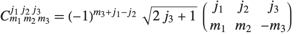 .
.
The 6‐j symbols SixJSymbol[{j1,j2,j3},{j4,j5,j6}] give the couplings of three quantum mechanical angular momentum states. The Racah coefficients are related by a phase to the 6‐j symbols.
ThreeJSymbol[{j, m}, {j + 1 / 2, -m - 1 / 2}, {1 / 2, 1 / 2}]| Exp[z] | exponential function |
| Log[z] | logarithm |
| Log[b,z] | logarithm |
| Log2[z]
,
Log10[z] | logarithm to base 2 and 10 |
| Sin[z]
,
Cos[z]
,
Tan[z]
,
Csc[z]
,
Sec[z]
,
Cot[z] | |
trigonometric functions (with arguments in radians)
| |
| ArcSin[z]
,
ArcCos[z]
,
ArcTan[z]
,
ArcCsc[z]
,
ArcSec[z]
,
ArcCot[z] | |
inverse trigonometric functions (giving results in radians)
| |
| ArcTan[x,y] | the argument of |
| Sinh[z]
,
Cosh[z]
,
Tanh[z]
,
Csch[z]
,
Sech[z]
,
Coth[z] | |
hyperbolic functions | |
| ArcSinh[z]
,
ArcCosh[z]
,
ArcTanh[z]
,
ArcCsch[z]
,
ArcSech[z]
,
ArcCoth[z] | |
inverse hyperbolic functions | |
| Sinc[z] | sinc function |
| Haversine[z] | haversine function |
| InverseHaversine[z] | inverse haversine function |
| Gudermannian[z] | Gudermannian function |
| InverseGudermannian[z] | inverse Gudermannian function |
Log[2, 1024]N[Log[2], 40]N[Log[-2]]N[Log[2 + 8 I]]Sin[Pi / 2]You can convert from degrees by explicitly multiplying by the constant Degree:
N[Sin[30 Degree]]Plot[Tanh[x], {x, -8, 8}]The haversine function Haversine[z] is defined by  . The inverse haversine function InverseHaversine[z] is defined by
  . The Gudermannian function Gudermannian[z] is defined as
 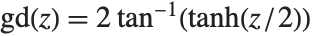 . The inverse Gudermannian function InverseGudermannian[z] is defined by
 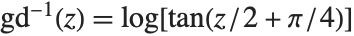 . The Gudermannian satisfies such relations as
 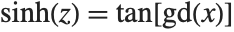 . The sinc function Sinc[z] is the Fourier transform of a square signal.
There are a number of additional trigonometric and hyperbolic functions that are sometimes used. The versine function is sometimes encountered in the literature and simply is  . The coversine function is defined as
  . The complex exponential
  is sometimes written as
  .
.
When you ask for the square root  of a number
  , you are effectively asking for the solution to the equation
  . This equation, however, in general has two different solutions. Both
  and
and  are, for example, solutions to the equation
  . When you evaluate the "function"
  , however, you usually want to get a single number, and so you have to choose one of these two solutions. A standard choice is that
  should be positive for
  . This is what the Wolfram Language function Sqrt[x] does.
The need to make one choice from two solutions means that Sqrt[x] cannot be a true inverse function for x^2. Taking a number, squaring it, and then taking the square root can give you a different number than you started with.
Sqrt[4]Sqrt[(-2) ^ 2]When you evaluate  , there are again two possible answers:
  and
and  . In this case, however, it is less clear which one to choose.
There is in fact no way to choose  so that it is continuous for all complex values of
  . There has to be a "branch cut"—a line in the complex plane across which the function
  is discontinuous. The Wolfram Language adopts the usual convention of taking the branch cut for
  to be along the negative real axis.
N[Sqrt[-2 I]]The branch cut in Sqrt along the negative real axis means that values of Sqrt[z] with  just above and below the axis are very different:
{Sqrt[-2 + 0.1 I], Sqrt[-2 - 0.1 I]}% ^ 2The discontinuity along the negative real axis is quite clear in this three‐dimensional picture of the imaginary part of the square root function:
Plot3D[Im[Sqrt[x + I y]], {x, -4, 4}, {y, -4, 4}]When you find an  th root using
  , there are, in principle,
  possible results. To get a single value, you have to choose a particular principal root. There is absolutely no guarantee that taking the
  th root of an
  th power will leave you with the same number.
(2.5 + I) ^ 10There are 10 possible tenth roots. The Wolfram Language chooses one of them. In this case it is not the number whose tenth power you took:
% ^ (1 / 10)There are many mathematical functions which, like roots, essentially give solutions to equations. The logarithm function and the inverse trigonometric functions are examples. In almost all cases, there are many possible solutions to the equations. Unique "principal" values nevertheless have to be chosen for the functions. The choices cannot be made continuous over the whole complex plane. Instead, lines of discontinuity, or branch cuts, must occur. The positions of these branch cuts are often quite arbitrary. The Wolfram Language makes the most standard mathematical choices for them.
| Sqrt[z] and z^s | |
| Exp[z] | none |
| Log[z] | |
trigonometric functions | none |
| ArcSin[z] and ArcCos[z] | |
| ArcTan[z] | |
| ArcCsc[z] and ArcSec[z] | |
| ArcCot[z] | |
hyperbolic functions | none |
| ArcSinh[z] | |
| ArcCosh[z] | |
| ArcTanh[z] | |
| ArcCsch[z] | |
| ArcSech[z] | |
| ArcCoth[z] |
ArcSin is a multiple‐valued function, so there is no guarantee that it always gives the "inverse" of Sin:
ArcSin[Sin[4.5]]Values of ArcSin[z] on opposite sides of the branch cut can be very different:
{ArcSin[2 + 0.1 I], ArcSin[2 - 0.1 I]}Plot3D[Im[ArcSin[x + I y]], {x, -4, 4}, {y, -4, 4}]| I | |
| Infinity | |
| Pi | |
| Degree | |
| GoldenRatio | |
| E | |
| EulerGamma | Euler's constant |
| Catalan | Catalan's constant |
| Khinchin | Khinchin's constant |
| Glaisher | Glaisher's constant |
Euler's constant EulerGamma is given by the limit  . It appears in many integrals, and asymptotic formulas. It is sometimes known as the Euler–Mascheroni constant, and denoted
  .
.
Catalan's constant Catalan is given by the sum  . It often appears in asymptotic estimates of combinatorial functions. It is variously denoted by
  ,
,  , or
, or  .
.
Khinchin's constant Khinchin (sometimes called Khintchine's constant) is given by  . It gives the geometric mean of the terms in the continued fraction representation for a typical real number.
Glaisher's constant Glaisher  (sometimes called the Glaisher–Kinkelin constant) satisfies
  , where
  is the Riemann zeta function. It appears in various sums and integrals, particularly those involving gamma and zeta functions.
N[EulerGamma, 40]IntegerPart[GoldenRatio ^ 100]| LegendreP[n,x] | Legendre polynomials |
| LegendreP[n,m,x] | associated Legendre polynomials |
| SphericalHarmonicY[l,m,θ,ϕ] | spherical harmonics |
| GegenbauerC[n,m,x] | Gegenbauer polynomials |
| ChebyshevT[n,x]
,
ChebyshevU[n,x] | Chebyshev polynomials |
| HermiteH[n,x] | Hermite polynomials |
| LaguerreL[n,x] | Laguerre polynomials |
| LaguerreL[n,a,x] | generalized Laguerre polynomials |
| ZernikeR[n,m,x] | Zernike radial polynomials |
| JacobiP[n,a,b,x] | Jacobi polynomials |
Legendre polynomials LegendreP[n,x] arise in studies of systems with three‐dimensional spherical symmetry. They satisfy the differential equation  , and the orthogonality relation
  for
for  .
.
The associated Legendre polynomials LegendreP[n,m,x] are obtained from derivatives of the Legendre polynomials according to  . Notice that for odd integers
  , the
, the  contain powers of
  , and are therefore not strictly polynomials. The
  reduce to
  when
when  .
.
The spherical harmonics SphericalHarmonicY[l,m,θ,ϕ] are related to associated Legendre polynomials. They satisfy the orthogonality relation  for
for  or
or  , where
  represents integration over the surface of the unit sphere.
LegendreP[8, x]Integrate[LegendreP[7, x] LegendreP[8, x], {x, -1, 1}]Integrate[LegendreP[8, x] ^ 2, {x, -1, 1}]Plot[LegendreP[10, x], {x, -1, 1}]LegendreP[8, 3, x]"Special Functions" discusses the generalization of Legendre polynomials to Legendre functions, which can have noninteger degrees:
LegendreP[8.1, 0]Gegenbauer polynomials GegenbauerC[n,m,x] can be viewed as generalizations of the Legendre polynomials to systems with  ‐dimensional spherical symmetry. They are sometimes known as ultraspherical polynomials.
GegenbauerC[n,0,x] is always equal to zero. GegenbauerC[n,x] is however given by the limit  . This form is sometimes denoted
  .
.
Series of Chebyshev polynomials are often used in making numerical approximations to functions. The Chebyshev polynomials of the first kind ChebyshevT[n,x] are defined by  . They are normalized so that
  . They satisfy the orthogonality relation
  for
for  . The
. The  also satisfy an orthogonality relation under summation at discrete points in
  corresponding to the roots of
  .
.
The Chebyshev polynomials of the second kind ChebyshevU[n,z] are defined by  . With this definition,
  . The
. The  satisfy the orthogonality relation
 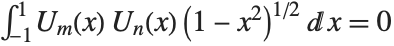 for
for  .
.
The name "Chebyshev" is a transliteration from the Cyrillic alphabet; several other spellings, such as "Tschebyscheff", are sometimes used.
Hermite polynomials HermiteH[n,x] arise as the quantum‐mechanical wave functions for a harmonic oscillator. They satisfy the differential equation 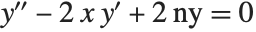 , and the orthogonality relation
 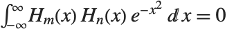 for
for  . An alternative form of Hermite polynomials sometimes used is
 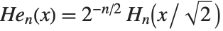 (a different overall normalization of the
  is also sometimes used).
This gives the density for an excited state of a quantum‐mechanical harmonic oscillator. The average of the wiggles is roughly the classical physics result:
Plot[(HermiteH[6, x] Exp[-x ^ 2 / 2]) ^ 2, {x, -6, 6}]Generalized Laguerre polynomials LaguerreL[n,a,x] are related to hydrogen atom wave functions in quantum mechanics. They satisfy the differential equation  , and the orthogonality relation
  for
for  . The Laguerre polynomials LaguerreL[n,x] correspond to the special case
  .
.
LaguerreL[2, a, x]Zernike radial polynomials ZernikeR[n,m,x] are used in studies of aberrations in optics. They satisfy the orthogonality relation  for
for  .
.
Jacobi polynomials JacobiP[n,a,b,x] occur in studies of the rotation group, particularly in quantum mechanics. They satisfy the orthogonality relation  for
for  . Legendre, Gegenbauer, Chebyshev and Zernike polynomials can all be viewed as special cases of Jacobi polynomials. The Jacobi polynomials are sometimes given in the alternative form
  .
.
The Wolfram System includes all the common special functions of mathematical physics found in standard handbooks. Each of the various classes of functions is discussed in turn.
One point you should realize is that in the technical literature there are often several conflicting definitions of any particular special function. When you use a special function in the Wolfram System, therefore, you should be sure to look at the definition given here to confirm that it is exactly what you want.
Gamma[15 / 2]Gamma[15 / 7]N[%, 40]Gamma[3 + 4I]//NGamma[{3 / 2, 5 / 2, 7 / 2}]D[Gamma[x], {x, 2}]You can use FindRoot to find roots of special functions:
FindRoot[BesselJ[0, x], {x, 1}]Special functions in the Wolfram System can usually be evaluated for arbitrary complex values of their arguments. Often, however, the defining relations given in this tutorial apply only for some special choices of arguments. In these cases, the full function corresponds to a suitable extension or analytic continuation of these defining relations. Thus, for example, integral representations of functions are valid only when the integral exists, but the functions themselves can usually be defined elsewhere by analytic continuation.
As a simple example of how the domain of a function can be extended, consider the function represented by the sum  . This sum converges only when
  . Nevertheless, it is easy to show analytically that for any
  , the complete function is equal to
  . Using this form, you can easily find a value of the function for any
  , at least so long as
  .
.
Gamma and Related Functions
| Beta[a,b] | Euler beta function |
| Beta[z,a,b] | incomplete beta function |
| BetaRegularized[z,a,b] | regularized incomplete beta function |
| Gamma[z] | Euler gamma function |
| Gamma[a,z] | incomplete gamma function |
| Gamma[a,z0,z1] | generalized incomplete gamma function |
| GammaRegularized[a,z] | regularized incomplete gamma function |
| InverseBetaRegularized[s,a,b] | inverse beta function |
| InverseGammaRegularized[a,s] | inverse gamma function |
| Pochhammer[a,n] | Pochhammer symbol |
| PolyGamma[z] | digamma function |
| PolyGamma[n,z] | |
| LogGamma[z] | Euler log-gamma function |
| LogBarnesG[z] | logarithm of Barnes G-function |
| BarnesG[z] | Barnes G-function |
| Hyperfactorial[n] | hyperfactorial function |
The Euler gamma function Gamma[z] is defined by the integral  . For positive integer
  ,
,  .
.  can be viewed as a generalization of the factorial function, valid for complex arguments
  .
.
There are some computations, particularly in number theory, where the logarithm of the gamma function often appears. For positive real arguments, you can evaluate this simply as Log[Gamma[z]]. For complex arguments, however, this form yields spurious discontinuities. The Wolfram System therefore includes the separate function LogGamma[z], which yields the logarithm of the gamma function with a single branch cut along the negative real axis.
The Pochhammer symbol or rising factorial Pochhammer[a,n] is  . It often appears in series expansions for hypergeometric functions. Note that the Pochhammer symbol has a definite value even when the gamma functions that appear in its definition are infinite.
The incomplete gamma function Gamma[a,z] is defined by the integral  . The Wolfram System includes a generalized incomplete gamma function Gamma[a,z0,z1] defined as
  .
.
The alternative incomplete gamma function  can therefore be obtained in the Wolfram System as Gamma[a,0,z].
The incomplete beta function Beta[z,a,b] is given by  . Notice that in the incomplete beta function, the parameter
  is an upper limit of integration, and appears as the first argument of the function. In the incomplete gamma function, on the other hand,
  is a lower limit of integration, and appears as the second argument of the function.
In certain cases, it is convenient not to compute the incomplete beta and gamma functions on their own, but instead to compute regularized forms in which these functions are divided by complete beta and gamma functions. The Wolfram System includes the regularized incomplete beta function BetaRegularized[z,a,b] defined for most arguments by  , but taking into account singular cases. The Wolfram System also includes the regularized incomplete gamma function GammaRegularized[a,z] defined by
  , with singular cases taken into account.
The incomplete beta and gamma functions, and their inverses, are common in statistics. The inverse beta function InverseBetaRegularized[s,a,b] is the solution for  in
in  . The inverse gamma function InverseGammaRegularized[a,s] is similarly the solution for
  in
in  .
.
Derivatives of the gamma function often appear in summing rational series. The digamma function PolyGamma[z] is the logarithmic derivative of the gamma function, given by  . For integer arguments, the digamma function satisfies the relation
  , where
  is Euler's constant (EulerGamma in the Wolfram System) and
  are the harmonic numbers.
The polygamma functions PolyGamma[n,z] are given by  . Notice that the digamma function corresponds to
  . The general form
  is the
  th, not the
  th, logarithmic derivative of the gamma function. The polygamma functions satisfy the relation
  . PolyGamma[ν,z] is defined for arbitrary complex
  by fractional calculus analytic continuation.
BarnesG[z] is a generalization of the Gamma function and is defined by its functional identity BarnesG[z+1]=Gamma[z] BarnesG[z], where the third derivative of the logarithm of BarnesG is positive for positive z. BarnesG is an entire function in the complex plane.
LogBarnesG[z] is a holomorphic function with a branch cut along the negative real-axis such that Exp[LogBarnesG[z]]=BarnesG[z].
PolyGamma[6]ContourPlot[Abs[Gamma[x + I y]], {x, -3, 3}, {y, -2, 2}, PlotPoints -> 50]Zeta and Related Functions
| DirichletL[k,j,s] | Dirichlet L-function |
| LerchPhi[z,s,a] | Lerch's transcendent |
| PolyLog[n,z] | polylogarithm function |
| PolyLog[n,p,z] | Nielsen generalized polylogarithm function |
| RamanujanTau[n] | Ramanujan |
| RamanujanTauL[n] | Ramanujan |
| RamanujanTauTheta[n] | Ramanujan |
| RamanujanTauZ[n] | Ramanujan |
| RiemannSiegelTheta[t] | Riemann–Siegel function |
| RiemannSiegelZ[t] | Riemann–Siegel function |
| StieltjesGamma[n] | Stieltjes constants |
| Zeta[s] | Riemann zeta function |
| Zeta[s,a] | generalized Riemann zeta function |
| HurwitzZeta[s,a] | Hurwitz zeta function |
| HurwitzLerchPhi[z,s,a] | Hurwitz–Lerch transcendent |
The Dirichlet-L function DirichletL[k,j,s] is implemented as  (for
(for  ) where
  is a Dirichlet character with modulus
  and index
  .
.
The Riemann zeta function Zeta[s] is defined by the relation  (for
(for  ). Zeta functions with integer arguments arise in evaluating various sums and integrals. The Wolfram System gives exact results when possible for zeta functions with integer arguments.
There is an analytic continuation of  for arbitrary complex
  . The zeta function for complex arguments is central to number theoretic studies of the distribution of primes. Of particular importance are the values on the critical line
  .
.
In studying  , it is often convenient to define the two Riemann–Siegel functions RiemannSiegelZ[t] and RiemannSiegelTheta[t] according to
  and
and  (for
(for  real). Note that the Riemann–Siegel functions are both real as long as
  is real.
The Stieltjes constants StieltjesGamma[n] are generalizations of Euler's constant that appear in the series expansion of  around its pole at
  ; the coefficient of
  is
is  . Euler's constant is
  .
.
The generalized Riemann zeta function Zeta[s,a] is implemented as  , where any term with
  is excluded.
The Ramanujan  Dirichlet L-function RamanujanTauL[s] is defined by L(s)
 (for
(for  ), with coefficients RamanujanTau[n]. In analogy with the Riemann zeta function, it is again convenient to define the functions RamanujanTauZ[t] and RamanujanTauTheta[t].
DirichletL[6, 2, 1. + I]Plot3D[Re@DirichletL[6, 2, u + I v], {u, -5, 5}, {v, -10, 10}, Mesh -> None, PlotStyle -> Directive[Opacity[0.7], Green, Specularity[10]], BoxRatios -> {1, 1, 2}]Zeta[6]Plot3D[Abs[Zeta[x + I y]], {x, -3, 3}, {y, 2, 35}]This is a plot of the absolute value of the Riemann zeta function on the critical line  . You can see the first few zeros of the zeta function:
Plot[Abs[Zeta[1 / 2 + I y]], {y, 0, 40}]Plot[Abs[RamanujanTauL[6 + I y]], {y, 0, 20}]The polylogarithm functions PolyLog[n,z] are given by  . The polylogarithm function is sometimes known as Jonquière's function. The dilogarithm PolyLog[2,z] satisfies
  . Sometimes
  is known as Spence's integral. The Nielsen generalized polylogarithm functions or hyperlogarithms PolyLog[n,p,z] are given by
  . Polylogarithm functions appear in Feynman diagram integrals in elementary particle physics, as well as in algebraic K‐theory.
The Lerch transcendent LerchPhi[z,s,a] is a generalization of the zeta and polylogarithm functions, given by  , where any term with
  is excluded. Many sums of reciprocal powers can be expressed in terms of the Lerch transcendent. For example, the Catalan beta function
  can be obtained as
  .
.
The Lerch transcendent is related to integrals of the Fermi–Dirac distribution in statistical mechanics by  .
.
The Lerch transcendent can also be used to evaluate Dirichlet L‐series that appear in number theory. The basic L‐series has the form  , where the "character"
  is an integer function with period
  . L‐series of this kind can be written as sums of Lerch functions with
  a power of
  .
.
The Hurwitz–Lerch transcendent HurwitzLerchPhi[z,s,a] generalizes HurwitzZeta[s,a] and is defined by  .
.
| ZetaZero[k] | the |
| ZetaZero[k,x0] | the |
Zeta[ZetaZero[1]]N[ZetaZero[1]]N[ZetaZero[1, 15]]Exponential Integral and Related Functions
| CosIntegral[z] | cosine integral function |
| CoshIntegral[z] | hyperbolic cosine integral function |
| ExpIntegralE[n,z] | exponential integral En(z) |
| ExpIntegralEi[z] | exponential integral |
| LogIntegral[z] | logarithmic integral |
| SinIntegral[z] | sine integral function |
| SinhIntegral[z] | hyperbolic sine integral function |
The second exponential integral function ExpIntegralEi[z] is defined by  (for
(for  ), where the principal value of the integral is taken.
The logarithmic integral function LogIntegral[z] is given by  (for
(for  ), where the principal value of the integral is taken.
  is central to the study of the distribution of primes in number theory. The logarithmic integral function is sometimes also denoted by
  . In some number theoretic applications,
  is defined as
  , with no principal value taken. This differs from the definition used in the Wolfram System by the constant
  .
.
The sine and cosine integral functions SinIntegral[z] and CosIntegral[z] are defined by  and
and  . The hyperbolic sine and cosine integral functions SinhIntegral[z] and CoshIntegral[z] are defined by
  and
and  .
.
Error Function and Related Functions
| Erf[z] | error function |
| Erf[z0,z1] | generalized error function |
| Erfc[z] | complementary error function |
| Erfi[z] | imaginary error function |
| FresnelC[z] | Fresnel integral C(z) |
| FresnelS[z] | Fresnel integral |
| InverseErf[s] | inverse error function |
| InverseErfc[s] | inverse complementary error function |
The error function Erf[z] is the integral of the Gaussian distribution, given by  . The complementary error function Erfc[z] is given simply by
  . The imaginary error function Erfi[z] is given by
  . The generalized error function Erf[z0,z1] is defined by the integral
  . The error function is central to many calculations in statistics.
The inverse error function InverseErf[s] is defined as the solution for  in the equation
  . The inverse error function appears in computing confidence intervals in statistics as well as in some algorithms for generating Gaussian random numbers.
Closely related to the error function are the Fresnel integrals FresnelC[z] defined by  and FresnelS[z] defined by
  . Fresnel integrals occur in diffraction theory.
Bessel and Related Functions
| AiryAi[z] and AiryBi[z] | Airy functions |
| AiryAiPrime[z] and AiryBiPrime[z] | derivatives of Airy functions |
| BesselJ[n,z] and BesselY[n,z] | Bessel functions |
| BesselI[n,z] and BesselK[n,z] | modified Bessel functions |
| KelvinBer[n,z] and KelvinBei[n,z] | Kelvin functions |
| KelvinKer[n,z] and KelvinKei[n,z] | Kelvin functions |
| HankelH1[n,z] and HankelH2[n,z] | Hankel functions |
| SphericalBesselJ[n,z] and SphericalBesselY[n,z] | |
spherical Bessel functions | |
| SphericalHankelH1[n,z] and SphericalHankelH2[n,z] | |
spherical Hankel functions | |
| StruveH[n,z] and StruveL[n,z] | Struve function |
The Bessel functions BesselJ[n,z] and BesselY[n,z] are linearly independent solutions to the differential equation 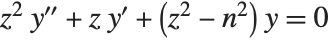 . For integer
  , the
, the  are regular at
  , while the
  have a logarithmic divergence at
  .
.
The Hankel functions (or Bessel functions of the third kind) HankelH1[n,z] and HankelH2[n,z] give an alternative pair of solutions to the Bessel differential equation, related according to 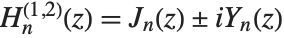 .
.
The spherical Bessel functions SphericalBesselJ[n,z] and SphericalBesselY[n,z], as well as the spherical Hankel functions SphericalHankelH1[n,z] and SphericalHankelH2[n,z], arise in studying wave phenomena with spherical symmetry. These are related to the ordinary functions by 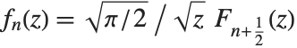 , where
  and
and  can be
  and
and  ,
,  and
and  , or
, or  and
and  . For integer
  , spherical Bessel functions can be expanded in terms of elementary functions by using FunctionExpand.
The modified Bessel functions BesselI[n,z] and BesselK[n,z] are solutions to the differential equation 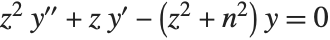 . For integer
  ,
,  is regular at
  ;
;  always has a logarithmic divergence at
  . The
. The  are sometimes known as hyperbolic Bessel functions.
Particularly in electrical engineering, one often defines the Kelvin functions KelvinBer[n,z], KelvinBei[n,z], KelvinKer[n,z] and KelvinKei[n,z]. These are related to the ordinary Bessel functions by  ,
,  .
.
The Airy functions AiryAi[z] and AiryBi[z] are the two independent solutions  and
and  to the differential equation
  .
.  tends to zero for large positive
  , while
  increases unboundedly. The Airy functions are related to modified Bessel functions with one‐third‐integer orders. The Airy functions often appear as the solutions to boundary value problems in electromagnetic theory and quantum mechanics. In many cases the derivatives of the Airy functions AiryAiPrime[z] and AiryBiPrime[z] also appear.
The Struve function StruveH[n,z] appears in the solution of the inhomogeneous Bessel equation, which for integer  has the form
  ; the general solution to this equation consists of a linear combination of Bessel functions with the Struve function
  added. The modified Struve function StruveL[n,z] is given in terms of the ordinary Struve function by
  . Struve functions appear particularly in electromagnetic theory.
Here is a plot of  . This is a curve that an idealized chain hanging from one end can form when you wiggle it:
Plot[BesselJ[0, Sqrt[x]], {x, 0, 50}]BesselK[3 / 2, x]The Airy function plotted here gives the quantum‐mechanical amplitude for a particle in a potential that increases linearly from left to right. The amplitude is exponentially damped in the classically inaccessible region on the right:
Plot[AiryAi[x], {x, -10, 10}]| BesselJZero[n,k] | the |
| BesselJZero[n,k,x0] | the |
| BesselYZero[n,k] | the |
| BesselYZero[n,k,x0] | the |
| AiryAiZero[k] | the |
| AiryAiZero[k,x0] | the |
| AiryBiZero[k] | the |
| AiryBiZero[k,x0] | the |
BesselJ[1, BesselJZero[1, 5]]N[BesselJZero[1, 5]]Legendre and Related Functions
| LegendreP[n,z] | Legendre functions of the first kind |
| LegendreP[n,m,z] | associated Legendre functions of the first kind |
| LegendreQ[n,z] | Legendre functions of the second kind |
| LegendreQ[n,m,z] | associated Legendre functions of the second kind |
The Legendre functions and associated Legendre functions satisfy the differential equation  . The Legendre functions of the first kind, LegendreP[n,z] and LegendreP[n,m,z], reduce to Legendre polynomials when
  and
and  are integers. The Legendre functions of the second kind LegendreQ[n,z] and LegendreQ[n,m,z] give the second linearly independent solution to the differential equation. For integer
  they have logarithmic singularities at
  . The
. The  and
and  solve the differential equation with
  .
.
| LegendreP[n,m,z] or LegendreP[n,m,1,z] | |
type 1 function containing | |
| LegendreP[n,m,2,z] | type 2 function containing |
| LegendreP[n,m,3,z] | type 3 function containing |
Types of Legendre functions. Analogous types exist for LegendreQ.
Legendre functions of type 1 and Legendre functions of type 2 have different symbolic forms, but the same numerical values. They have branch cuts from  to
to  and from
  to
to  . Legendre functions of type 3, sometimes denoted
  and
and  , have a single branch cut from
  to
to  .
.
Toroidal functions or ring functions, which arise in studying systems with toroidal symmetry, can be expressed in terms of the Legendre functions  and
and  .
.
When you use the function LegendreP[n,x] with an integer  , you get a Legendre polynomial. If you take
  to be an arbitrary complex number, you get, in general, a Legendre function.
In the same way, you can use the functions GegenbauerC and so on with arbitrary complex indices to get Gegenbauer functions, Chebyshev functions, Hermite functions, Jacobi functions and Laguerre functions. Unlike for associated Legendre functions, however, there is no need to distinguish different types in such cases.
Hypergeometric Functions and Generalizations
| Hypergeometric0F1[a,z] | hypergeometric function |
| Hypergeometric0F1Regularized[a,z] | regularized hypergeometric function |
| Hypergeometric1F1[a,b,z] | Kummer confluent hypergeometric function |
| Hypergeometric1F1Regularized[a,b,z] | regularized confluent hypergeometric function |
| HypergeometricU[a,b,z] | confluent hypergeometric function |
| WhittakerM[k,m,z] and WhittakerW[k,m,z] | |
Whittaker functions | |
| ParabolicCylinderD[ν,z] | parabolic cylinder function |
| CoulombF[l,η,ρ] | regular Coulomb wavefunction |
| CoulombG[l,η,ρ] | irregular Coulomb wavefunction |
Many of the special functions that have been discussed so far can be viewed as special cases of the confluent hypergeometric function Hypergeometric1F1[a,b,z].
The confluent hypergeometric function can be obtained from the series expansion  . Some special results are obtained when
  and
and  are both integers. If
  , and either
  or
or  , the series yields a polynomial with a finite number of terms.
If  is zero or a negative integer, then
  itself is infinite. But the regularized confluent hypergeometric function Hypergeometric1F1Regularized[a,b,z] given by
  has a finite value in all cases.
Among the functions that can be obtained from  are the Bessel functions, error function, incomplete gamma function, and Hermite and Laguerre polynomials.
The  confluent hypergeometric function is a solution to Kummer's differential equation
  , with the boundary conditions
  and
and  .
.
The function HypergeometricU[a,b,z] gives a second linearly independent solution to Kummer's equation. For  this function behaves like
  for small
  . It has a branch cut along the negative real axis in the complex
  plane.
The Whittaker functions WhittakerM[k,m,z] and WhittakerW[k,m,z] give a pair of solutions to the normalized Kummer differential equation, known as Whittaker's differential equation. The Whittaker function  is related to
  by
by  . The second Whittaker function
  obeys the same relation, with
  replaced by
  .
.
The Coulomb wavefunctions CoulombF[l,η,ρ] and CoulombG[l,η,ρ] are also special cases of the confluent hypergeometric function. Coulomb wavefunctions give solutions to the radial Schrödinger equation in the Coulomb potential of a point nucleus. The regular Coulomb wavefunction is given by  , where
  . The irregular Coulomb wavefunction
  is given by a similar expression, with
  replaced by
  .
.
The outgoing and incoming irregular Coulomb wavefunctions CoulombH1[l,η,ρ] and CoulombH2[l,η,ρ] are a linear combination of the regular and irregular Coulomb wavefunctions, related according to  .
.
Other special cases of the confluent hypergeometric function include the Toronto functions  , Poisson–Charlier polynomials
  , Cunningham functions
  , and Bateman functions
  .
.
A limiting form of the confluent hypergeometric function that often appears is Hypergeometric0F1[a,z]. This function is obtained as the limit  .
.
| Hypergeometric2F1[a,b,c,z] | hypergeometric function |
| Hypergeometric2F1Regularized[a,b,c,z] | |
regularized hypergeometric function | |
| HypergeometricPFQ[{a1,…,ap},{b1,…,bq},z] | |
generalized hypergeometric function | |
| HypergeometricPFQRegularized[{a1,…,ap},{b1,…,bq},z] | |
regularized generalized hypergeometric function | |
| MeijerG[{{a1,…,an},{an+1,…,ap}},{{b1,…,bm},{bm+1,…,bq}},z] | |
Meijer G-function | |
| AppellF1[a,b1,b2,c,x,y] | Appell hypergeometric function of two variables |
The hypergeometric function Hypergeometric2F1[a,b,c,z] has series expansion  . The function is a solution of the hypergeometric differential equation
  .
.
The hypergeometric function is also sometimes denoted by  , and is known as the Gauss series or the Kummer series.
The Legendre functions, and the functions that give generalizations of other orthogonal polynomials, can be expressed in terms of the hypergeometric function. Complete elliptic integrals can also be expressed in terms of the  function.
The Riemann P function, which gives solutions to Riemann's differential equation, is also a  function.
The generalized hypergeometric function or Barnes extended hypergeometric function HypergeometricPFQ[{a1,…,ap},{b1,…,bq},z] has series expansion 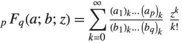 .
.
The Meijer G-function MeijerG[{{a1,…,an},{an+1,…,ap}},{{b1,…,bm},{bm+1,…,bq}},z] is defined by the contour integral representation 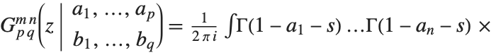
 , where the contour of integration is set up to lie between the poles of
  and the poles of
  . MeijerG is a very general function whose special cases cover most of the functions discussed in the past few sections.
The Appell hypergeometric function of two variables AppellF1[a,b1,b2,c,x,y] has series expansion  . This function appears for example in integrating cubic polynomials to arbitrary powers.
The q-Series and Related Functions
| QPochhammer[z,q] | |
| QPochhammer[z,q,n] | |
| QFactorial[z,q] | |
| QBinomial[n,m,q] | |
| QGamma[z,q] | |
| QPolyGamma[z,q] | |
| QPolyGamma[n,z,q] | |
| QHypergeometricPFQ[{a1,…,ap},{b1,…,bq},q,z] | |
basic hypergeometric series | |
The  -Pochhammer symbol is a natural object in the calculus of
  -differences, playing the same role as the power function in infinitesimal calculus or the falling factorial in the calculus of finite differences.
The finite  -Pochhammer symbol
  is defined as the product
  . The limit
  defines the
  -Pochhammer symbol
  when
when  <1. The
  -Pochhammer symbol
  is the
  -analog of the Pochhammer
  symbol, which is recovered in the limit

 /(1-q)n.
The  -factorial
  is defined as
  /(1-q)z and is a
  -analog of the factorial function, which is recovered as
  . The relationship
 between the
  -factorial and the
  -gamma functions has the same functional form as the relationship z!
 between the factorial and the Euler gamma function.
The  -digamma function is defined as the logarithmic derivative of the
  -gamma function

 . The
. The  -polygamma function
  of order
  is defined as the
  th derivative with respect to
  of the
  -digamma function.
The basic hypergeometric series is a  -analog of the generalized hypergeometric series. It was introduced by Heine as a
  -analog of Gauss hypergeometric series and arises in combinatorics.
The Product Log Function
| ProductLog[z] | product log function |
The product log function gives the solution for  in
in  . The function can be viewed as a generalization of a logarithm. It can be used to represent solutions to a variety of transcendental equations. The tree generating function for counting distinct oriented trees is related to the product log by
  .
.
Spheroidal Functions
| SpheroidalS1[n,m,γ,z] and SpheroidalS2[n,m,γ,z] | |
radial spheroidal functions | |
| SpheroidalS1Prime[n,m,γ,z] and SpheroidalS2Prime[n,m,γ,z] | |
z derivatives of radial spheroidal functions | |
| SpheroidalPS[n,m,γ,z] and SpheroidalQS[n,m,γ,z] | |
angular spheroidal functions | |
| SpheroidalPSPrime[n,m,γ,z] and SpheroidalQSPrime[n,m,γ,z] | |
z derivatives of angular spheroidal functions | |
| SpheroidalEigenvalue[n,m,γ] | spheroidal eigenvalue of degree n and order m |
The radial spheroidal functions SpheroidalS1[n,m,γ,z] and SpheroidalS2[n,m,γ,z] and angular spheroidal functions SpheroidalPS[n,m,γ,z] and SpheroidalQS[n,m,γ,z] appear in solutions to the wave equation in spheroidal regions. Both types of functions are solutions to the equation  . This equation has normalizable solutions only when
  is a spheroidal eigenvalue given by SpheroidalEigenvalue[n,m,γ]. The spheroidal functions also appear as eigenfunctions of finite analogs of Fourier transforms.
SpheroidalS1 and SpheroidalS2 are effectively spheroidal analogs of the spherical Bessel functions  and
and  , while SpheroidalPS and SpheroidalQS are effectively spheroidal analogs of the Legendre functions
  and
and  .
.  corresponds to a prolate spheroidal geometry, while
  corresponds to an oblate spheroidal geometry.
Many different normalizations for spheroidal functions are used in the literature. The Wolfram System uses the Meixner–Schäfke normalization scheme.
Series[SpheroidalPS[n, 0, γ, η], {γ, 0, 3}]Plot[{SpheroidalPS[3, 0, 0, η], SpheroidalPS[3, 0, 3, η], SpheroidalPS[3, 0, 5, η]}, {η, -1, 1}]Integrate[SpheroidalPS[3, 0, γ, η]Exp[I ω γ η], {η, -1, 1}]SpheroidalPS[1 / 2, 1 / 2, c, z]Even more so than for other special functions, you need to be very careful about the arguments you give to elliptic integrals and elliptic functions. There are several incompatible conventions in common use, and often these conventions are distinguished only by the specific names given to arguments or by the presence of separators other than commas between arguments.
■ Amplitude |
■ Argument |
■ Delta amplitude |
■ Coordinate |
■ Characteristic |
■ Parameter |
■ Complementary parameter |
■ Modulus |
■ Modular angle |
■ Nome |
■ Invariants |
■ Half‐periods |
■ Ratio of periods |
■ Discriminant |
■ Parameters of curve |
■ Coordinate |
| JacobiAmplitude[u,m] | give the amplitude ϕ corresponding to argument u and parameter m |
| EllipticNomeQ[m] | give the nome q corresponding to parameter m |
| InverseEllipticNomeQ[q] | give the parameter m corresponding to nome q |
| WeierstrassInvariants[{ω,ω′}] | give the invariants {g2,g3} corresponding to the half‐periods {ω,ω′} |
| WeierstrassHalfPeriods[{g2,g3}] | give the half‐periods {ω,ω′} corresponding to the invariants {g2,g3} |
Elliptic Integrals
| EllipticK[m] | complete elliptic integral of the first kind |
| EllipticF[ϕ,m] | elliptic integral of the first kind |
| EllipticE[m] | complete elliptic integral of the second kind E(m) |
| EllipticE[ϕ,m] | elliptic integral of the second kind E(ϕm) |
| EllipticPi[n,m] | complete elliptic integral of the third kind |
| EllipticPi[n,ϕ,m] | elliptic integral of the third kind |
| JacobiZeta[ϕ,m] | Jacobi zeta function |
Integrals of the form  , where
  is a rational function, and
  is a cubic or quartic polynomial in
  , are known as elliptic integrals. Any elliptic integral can be expressed in terms of the three standard kinds of Legendre–Jacobi elliptic integrals.
The elliptic integral of the first kind EllipticF[ϕ,m] is given for  by
by 
 . This elliptic integral arises in solving the equations of motion for a simple pendulum. It is sometimes known as an incomplete elliptic integral of the first kind.
Note that the arguments of the elliptic integrals are sometimes given in the opposite order from what is used in the Wolfram Language.
The complete elliptic integral of the first kind EllipticK[m] is given by  . Note that
  is used to denote the complete elliptic integral of the first kind, while
  is used for its incomplete form. In many applications, the parameter
  is not given explicitly, and
  is denoted simply by
  . The complementary complete elliptic integral of the first kind
  is given by
  . It is often denoted
  .
.  and
and  give the "real" and "imaginary" quarter‐periods of the corresponding Jacobi elliptic functions discussed in "Elliptic Functions".
The complete elliptic integral of the second kind EllipticE[m] is given by  . It is often denoted
  . The complementary form is
  .
.
Plot[EllipticE[m], {m, 0, 1}]EllipticK[Sin[30 Degree] ^ 2]//NPlot3D[Im[EllipticF[px + I py, 2]], {px, 0.5, 2.5}, {py, -1, 1}, PlotPoints -> 60]Elliptic Functions
| JacobiAmplitude[u,m] | amplitude function |
| JacobiSN[u,m]
,
JacobiCN[u,m]
, etc.
| |
Jacobi elliptic functions | |
| InverseJacobiSN[v,m]
,
InverseJacobiCN[v,m]
, etc.
| |
inverse Jacobi elliptic functions | |
| EllipticTheta[a,u,q] | theta functions |
| EllipticThetaPrime[a,u,q] | derivatives of theta functions |
| SiegelTheta[τ,s] | Siegel theta function |
| SiegelTheta[v,τ,s] | Siegel theta function |
| WeierstrassP[u,{g2,g3}] | Weierstrass elliptic function |
| WeierstrassPPrime[u,{g2,g3}] | derivative of Weierstrass elliptic function |
| InverseWeierstrassP[p,{g2,g3}] | inverse Weierstrass elliptic function |
| WeierstrassSigma[u,{g2,g3}] | Weierstrass sigma function |
| WeierstrassZeta[u,{g2,g3}] | Weierstrass zeta function |
Rational functions involving square roots of quadratic forms can be integrated in terms of inverse trigonometric functions. The trigonometric functions can thus be defined as inverses of the functions obtained from these integrals.
By analogy, elliptic functions are defined as inverses of the functions obtained from elliptic integrals.
The amplitude for Jacobi elliptic functions JacobiAmplitude[u,m] is the inverse of the elliptic integral of the first kind. If  , then
  . In working with Jacobi elliptic functions, the argument
  is often dropped, so
  is written as
  .
.
The Jacobi elliptic functions JacobiSN[u,m] and JacobiCN[u,m] are given respectively by  and
and  , where
  . In addition, JacobiDN[u,m] is given by
  .
.
There are a total of twelve Jacobi elliptic functions JacobiPQ[u,m], with the letters P and Q chosen from the set S, C, D and N. Each Jacobi elliptic function JacobiPQ[u,m] satisfies the relation  , where for these purposes
  .
.
There are many relations between the Jacobi elliptic functions, somewhat analogous to those between trigonometric functions. In limiting cases, in fact, the Jacobi elliptic functions reduce to trigonometric functions. So, for example,  ,
,  ,
,  ,
,  ,
,  and
and  .
.
The notation  is often used for the integrals
  . These integrals can be expressed in terms of the Jacobi zeta function defined in "Elliptic Integrals".
One of the most important properties of elliptic functions is that they are doubly periodic in the complex values of their arguments. Ordinary trigonometric functions are singly periodic, in the sense that  for any integer
  . The elliptic functions are doubly periodic, so that
  for any pair of integers
  and
and  .
.
The Jacobi elliptic functions  , etc. are doubly periodic in the complex
  plane. Their periods include
  and
and  , where
  is the complete elliptic integral of the first kind.
The choice of "p" and "q" in the notation  for Jacobi elliptic functions can be understood in terms of the values of the functions at the quarter periods
  and
and  .
.
This shows two complete periods in each direction of the absolute value of the Jacobi elliptic function  :
:
ContourPlot[Abs[JacobiSN[ux + I uy, 1 / 3]], {ux, 0, 4 EllipticK[1 / 3]}, {uy, 0, 4 EllipticK[2 / 3]}]Also built into the Wolfram Language are the inverse Jacobi elliptic functions InverseJacobiSN[v,m], InverseJacobiCN[v,m], etc. The inverse function  , for example, gives the value of
  for which
  . The inverse Jacobi elliptic functions are related to elliptic integrals.
The four theta functions  are obtained from EllipticTheta[a,u,q] by taking a to be 1, 2, 3, or 4. The functions are defined by
  ,
,  ,
, 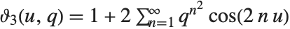 ,
,  . The theta functions are often written as
  with the parameter
  not explicitly given. The theta functions are sometimes written in the form
  , where
  is related to
  by
by  . In addition,
  is sometimes replaced by
  , given by
  . All the theta functions satisfy a diffusion‐like differential equation
 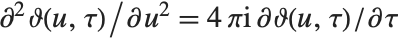 .
.
The Siegel theta function SiegelTheta[τ,s] with Riemann square modular matrix  of dimension p and vector s generalizes the elliptic theta functions to complex dimension p. It is defined by
  , where n runs over all p-dimensional integer vectors. The Siegel theta function with characteristic SiegelTheta[ν,τ,s] is defined by
  , where the characteristic ν is a pair of p-dimensional vectors {α,β}.
The Neville theta functions can be defined in terms of the theta functions as 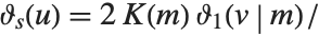
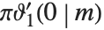 ,
, 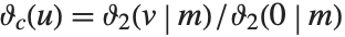 ,
, 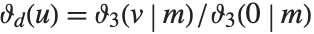 ,
,  , where
  . The Jacobi elliptic functions can be represented as ratios of the Neville theta functions.
The Weierstrass elliptic function WeierstrassP[u,{g2,g3}] can be considered as the inverse of an elliptic integral. The Weierstrass function  gives the value of
  for which
  . The function WeierstrassPPrime[u,{g2,g3}] is given by
  .
.
The Weierstrass functions are also sometimes written in terms of their fundamental half‐periods  and
and  , obtained from the invariants
  and
and  using WeierstrassHalfPeriods[{g2,g3}].
The function InverseWeierstrassP[p,{g2,g3}] finds one of the two values of  for which
  . This value always lies in the parallelogram defined by the complex number half‐periods
  and
and  .
.
InverseWeierstrassP[{p,q},{g2,g3}] finds the unique value of  for which
  and
and  . In order for any such value of
  to exist,
  and
and  must be related by
  .
.
The Weierstrass zeta function WeierstrassZeta[u,{g2,g3}] and Weierstrass sigma function WeierstrassSigma[u,{g2,g3}] are related to the Weierstrass elliptic functions by  and
and  .
.
The Weierstrass zeta and sigma functions are not strictly elliptic functions since they are not periodic.
Elliptic Modular Functions
| DedekindEta[τ] | Dedekind eta function |
| KleinInvariantJ[τ] | Klein invariant modular function |
| ModularLambda[τ] | modular lambda function |
The modular lambda function ModularLambda[τ] relates the ratio of half‐periods  to the parameter according to
  .
.
The Klein invariant modular function KleinInvariantJ[τ] and the Dedekind eta function DedekindEta[τ] satisfy the relations  .
.
Modular elliptic functions are defined to be invariant under certain fractional linear transformations of their arguments. Thus for example  is invariant under any combination of the transformations
  and
and  .
.
Generalized Elliptic Integrals and Functions
| ArithmeticGeometricMean[a,b] | the arithmetic‐geometric mean of |
| EllipticExp[u,{a,b}] | generalized exponential associated with the elliptic curve |
| EllipticLog[{x,y},{a,b}] | generalized logarithm associated with the elliptic curve |
The definitions for elliptic integrals and functions given above are based on traditional usage. For modern algebraic geometry, it is convenient to use slightly more general definitions.
The function EllipticLog[{x,y},{a,b}] is defined as the value of the integral  , where the sign of the square root is specified by giving the value of
  such that
  . Integrals of the form
  can be expressed in terms of the ordinary logarithm (and inverse trigonometric functions). You can think of EllipticLog as giving a generalization of this, where the polynomial under the square root is now of degree three.
The function EllipticExp[u,{a,b}] is the inverse of EllipticLog. It returns the list {x,y} that appears in EllipticLog. EllipticExp is an elliptic function, doubly periodic in the complex  plane.
ArithmeticGeometricMean[a,b] gives the arithmetic‐geometric mean (AGM) of two numbers  and
and  . This quantity is central to many numerical algorithms for computing elliptic integrals and other functions. For positive reals
  and
and  the AGM is obtained by starting with
  ,
,  , then iterating the transformation
  ,
,  until
until  to the precision required.
| MathieuC[a,q,z] | even Mathieu functions with characteristic value a and parameter q |
| MathieuS[b,q,z] | odd Mathieu functions with characteristic value b and parameter q |
| MathieuCPrime[a,q,z] and MathieuSPrime[b,q,z] | z derivatives of Mathieu functions |
| MathieuCharacteristicA[r,q] | characteristic value ar for even Mathieu functions with characteristic exponent r and parameter q |
| MathieuCharacteristicB[r,q] | characteristic value br for odd Mathieu functions with characteristic exponent r and parameter q |
| MathieuCharacteristicExponent[a,q] | characteristic exponent r for Mathieu functions with characteristic value a and parameter q |
The Mathieu functions MathieuC[a,q,z] and MathieuS[a,q,z] are solutions to the equation  . This equation appears in many physical situations that involve elliptical shapes or periodic potentials. The function MathieuC is defined to be even in
  , while MathieuS is odd.
When  the Mathieu functions are simply
  and
and  . For nonzero
  , the Mathieu functions are only periodic in
  for certain values of
  . Such Mathieu characteristic values are given by MathieuCharacteristicA[r,q] and MathieuCharacteristicB[r,q] with
  an integer or rational number. These values are often denoted by
  and
and  .
.
For integer  , the even and odd Mathieu functions with characteristic values
  and
and  are often denoted
  and
and  , respectively. Note the reversed order of the arguments
  and
and  .
.
According to Floquet's theorem, any Mathieu function can be written in the form  , where
  has period
  and
and  is the Mathieu characteristic exponent MathieuCharacteristicExponent[a,q]. When the characteristic exponent
  is an integer or rational number, the Mathieu function is therefore periodic. In general, however, when
  is not a real integer,
  and
and  turn out to be equal.
Plot[Evaluate[Table[MathieuCharacteristicA[r, q], {r, 0, 4}]], {q, 0, 15}]automatic evaluation | exact results for specific arguments |
| N[expr,n] | numerical approximations to any precision |
| D[expr,x] | exact results for derivatives |
| N[D[expr,x]] | numerical approximations to derivatives |
| Series[expr,{x,x0,n}] | series expansions |
| Integrate[expr,x] | exact results for integrals |
| NIntegrate[expr,x] | numerical approximations to integrals |
| FindRoot[expr==0,{x,x0}] | numerical approximations to roots |
Most special functions have simpler forms when given certain specific arguments. The Wolfram System will automatically simplify special functions in such cases.
PolyLog[2, 1 / 2]Here again the Wolfram System reduces a special case of the Airy function to an expression involving gamma functions:
AiryAi[0]For most choices of arguments, no exact reductions of special functions are possible. But in such cases, the Wolfram System allows you to find numerical approximations to any degree of precision. The algorithms that are built into the Wolfram System cover essentially all values of parameters—real and complex—for which the special functions are defined.
AiryAi[1]N[AiryAi[1], 40]N[AiryAi[1000 I]]Most special functions have derivatives that can be expressed in terms of elementary functions or other special functions. But even in cases where this is not so, you can still use N to find numerical approximations to derivatives.
D[FresnelS[x], x]Gamma'[3]Zeta'[Pi]Applying N gives a numerical approximation:
N[%]The Wolfram System incorporates a vast amount of knowledge about special functions—including essentially all the results that have been derived over the years. You access this knowledge whenever you do operations on special functions in the Wolfram System.
Series[FresnelS[x], {x, 0, 15}]Integrate[AiryAi[x] ^ 2, {x, 0, Infinity}]One feature of working with special functions is that there are a large number of relations between different functions, and these relations can often be used in simplifying expressions.
| FullSimplify[expr] | try to simplify expr using a range of transformation rules |
FullSimplify[Gamma[x] Gamma[1 - x]]FullSimplify[ChebyshevT[n, z] - k Cos[n ArcCos[z]]]FullSimplify[3 AiryAi[1] + Sqrt[3] AiryBi[1]]| FunctionExpand[expr] | try to expand out special functions |
FunctionExpand[Hypergeometric2F1[1 / 2, 3 / 2, 3, x]]FunctionExpand[BesselY[n, I x]]In this case the final result does not even involve PolyGamma:
FunctionExpand[Im[PolyGamma[0, 3 I]]]FunctionExpand[Derivative[1, 0][Zeta][-1, 4]]