数学函数
| 命名规则 | 多值函数 |
| 一般和非一般情况 | 数学常数 |
| 数值函数 | 正交多项式 |
| 分段函数 | 特殊函数 |
| 伪随机数 | 椭圆积分和椭圆函数 |
| 整数和数论中的函数 | Mathieu 函数和相关的函数 |
| 组合函数 | 带有特殊函数的运算 |
| 初等超越函数 |
Wolfram 语言中的数学函数根据定义规则来命名. 对大多数 Wolfram 语言函数,名称通常是完整的完全拼写的英语单词. 对于一些很常见的函数,Wolfram 语言使用传统缩写. 例如,模函数的名称是 Mod,而不是 Modulo.
通常涉及人的名字的数学函数在 Wolfram 语言中有形如 PersonSymbol 的名称. 例如,勒让德多项式  被表示为LegendreP[n,x]. 尽管这个惯例使函数的名称较长,但它避免了任何模棱两可或混乱不清.
| IntegerPart[x] | x 的整数部分 |
| FractionalPart[x] | x 的分数部分 |
| Round[x] | 最接近 x 的整数 〈x〉 |
| Floor[x] | 小于等于 x 的最大整数 ⌊x⌋ |
| Ceiling[x] | 大于等于 x 的最小整数 ⌈x⌉ |
| Rationalize[x] | 近似于 x 的有理数 |
| Rationalize[x,dx] | 容差 dx 内的有理数近似 |
| x | IntegerPart[x] | FractionalPart[x] | Round[x] | Floor[x] | Ceiling[x] |
| 2.4 | 2 | 0.4 | 2 | 2 | 3 |
| 2.5 | 2 | 0.5 | 2 | 2 | 3 |
| 2.6 | 2 | 0.6 | 3 | 2 | 3 |
| -2.4 | -2 | -0.4 | -2 | -3 | -2 |
| -2.5 | -2 | -0.5 | -2 | -3 | -2 |
| -2.6 | -2 | -0.6 | -3 | -3 | -2 |
IntegerPart[x] 和 FractionalPart[x] 可以看作是提取小数点左边和右边的数字. Round[x] 常被用来强迫接近整数的一个数成为真正的整数. Floor[x] 和 Ceiling[x] 常出现在计算一个具有非整数间隔的数列中有多少元素的事项中.
| RealSign[x] | 对于 x>0 为 1;对于 x<0 为 -1 |
| UnitStep[x] | 对于 x≥0 为 1;对于 x<0 为 0 |
| RealAbs[x] | x 的绝对值 x |
| Clip[x] | 介于 ‐1 和 +1 之间的 x |
| Rescale[x,{xmin,xmax}] | 重新调整为从 0 到 1 的 x |
| Max[x1,x2,…] or Max[{x1,x2,…},…] | |
x1, x2, … 的最大值 | |
| Min[x1,x2,…] or Min[{x1,x2,…},…] | |
x1, x2, … 的最小值 | |
| x+I y | 复数 x+iy |
| Re[z] | 实部 Re z |
| Im[z] | 虚部 Im z |
| Conjugate[z] | 多共轭 z* 或 |
| Abs[z] | 绝对值 z |
| Arg[z] | 幅角 ϕ 使得 z=zei ϕ |
| Sign[z] | z≠0 时,复数 sign z/z |
经常地,在不同区域中具有不同形式的函数是很方便的. 这可以使用 Piecewise 来实现.
分段函数出现在在不同区域离散切换的系统中. 它们也是许多计算方法的核心,包括样条(splines)和有限元(finite elements). 特殊情况包括这样的函数如 Abs、UnitStep、Clip、Sign、Floor 和 Max. Wolfram 语言处理符号和数值两种情况下的分段函数.
| RandomInteger[] | 概率为 |
| RandomInteger[{imin,imax}] | 包含在 imin 和 imax 内的伪随机整数 |
| RandomInteger[imax] | 包含在 0 和 imax 内的伪随机整数 |
| RandomReal[ ] | 0 和 1 之间的伪随机实数 |
| RandomReal[{xmin, xmax}] | xmin 和 xmax 之间的伪随机实数 |
| RandomReal[xmax] | 0 和 xmax 之间的伪随机实数 |
| RandomComplex[] | 单位方域中的伪随机复数 |
| RandomComplex[{zmin,zmax}] | 由 zmin 和 zmax 定义的长方形中的伪随机复数 |
| RandomComplex[zmax] | 由 0 和 zmax 定义的长方形中的伪随机复数 |
| RandomReal[range,n]
,
RandomComplex[range,n]
,
RandomInteger[range,n] | |
从给定区域得到的 n 个伪随机数的列表 | |
| RandomReal[range,{n1,n2,…}]
,
RandomComplex[range,{n1,n2,…}]
,
RandomInteger[range,{n1,n2,…}] | |
由伪随机数组成的 n1×n2×… 数组 | |
选项名
|
默认值
| |
| WorkingPrecision | MachinePrecision | 用于实数或者复数的精度 |
使用伪随机数的一个常见方法是进行数值假设检验. 例如,如果用户相信两个符号表达式在数学上是相等的. 可以通过给符号参数插上“典型”数值的值. 然后比较数值结果来进行检验. (如果要这样做的话,在数值准确度问题上,在可能没有唯一值的复变量的函数上,都应当仔细注意).
用随机数字代入表明方程不总是为真 True:
RandomInteger、RandomReal 和 RandomComplex 与其他的 Wolfram 语言函数不同,每次调用它时,都将得到不同的结果. 因此,如果在计算中使用它们,在不同的时机会得到不同的答案.
由 RandomInteger、RandomReal 和 RandomComplex 得到的序列在多数意义下并不是“真正随机的”,尽管实际上它们应当是“足够随机的”. 事实上,这个序列是通过使用从一个特定起点开始的确定数学算法生成的. 如果给出相同的起点,将得到相同的序列.
如果用户想要确定总是得到相同的伪随机数序列,可以使用 SeedRandom 明显地给伪随机数生成一个起点.
| SeedRandom[] | 使用时钟时刻重设伪随机生成器的起点 |
| SeedRandom[s] | 使用整数 s 重设伪随机生成器的起点 |
每调用一次 RandomInteger、RandomReal 或者 RandomComplex,伪随机数生成器的内部状态就被改变,这意味着在辅助运算中调用这些函数,将会影响主运算中返回的数. 要避免这个问题,可以在运算 BlockRandom 中局部化这些函数的使用效果.
| BlockRandom[expr] | 使用局部化的伪随机生成器的当前状态计算 expr |
通过在 BlockRandom 中进行局部化计算,在生成第一个列表之后,伪随机数生成器的状态被恢复:
| RandomInteger[dist]
,
RandomReal[dist] | |
服从随机分布 dist 的伪随机数 | |
| RandomInteger[dist,n]
,
RandomReal[dist,n] | |
服从随机分布 dist 的 n 个伪随机数的列表 | |
| RandomInteger[dist,{n1,n2,…}]
,
RandomReal[dist,{n1,n2,…}] | |
由服从随机分布 dist 的伪随机数组成的 n1×n2×… 数组 | |
| RandomChoice[list, n] | 从 list 随机选择 n 个项 |
| RandomChoice[list,{n1,n2,…}] | 从 list 随机选择得到的值组成的 n1×n2×… 数组 |
| RandomSample[list, n] | 从 list 得到的大小为 n 的样本 |
| Mod[k,n] | k 模 n ( k 除以 n 的余数) |
| Quotient[m,n] | m 和 n 的商 ( m/n 的整数部分) |
| QuotientRemainder[m,n] | 商和余数的列表 |
| Divisible[m,n] | 检测 m 是否被 n 整除 |
| CoprimeQ[n1,n2,…] | 检测 ni 是否成对互质 |
| GCD[n1,n2,…] | n1, n2, … 的最大公约数 |
| LCM[n1,n2,…] | n1, n2, … 的最小公倍数 |
| KroneckerDelta[n1,n2,…] | 如果所有的 ni 都相等,那么 Kronecker delta |
| IntegerDigits[n,b] | b 进制下 n 的位数 |
| IntegerExponent[n,b] | 整除 n 的 b 次幂的最大值 |
Mod 也可用于实数:
由 Mod 得到的结果,其符号与第二个自变量的符号相同:
| Mod[k,n] | 结果在 0 到 n-1 之间 |
| Mod[k,n,1] | 结果在 1 到 n 之间 |
| Mod[k,n,-n/2] | 结果在 ⌈-n/2⌉ 到 ⌊+n/2⌋ 之间 |
| Mod[k,n,d] | 结果在 d 到 d+n-1 之间 |
特别当使用 Mod 来获得部分对象的索引时,指定一个偏心距常常是方便的.
| FactorInteger[n] | n 的素因子和相应指数的列表 |
| Divisors[n] | 整除 n 的整数列表 |
| Prime[k] | 第 k 个素数 |
| PrimePi[x] | 第 k 个素数 |
| PrimeQ[n] | |
| PrimeNu[n] | n 中不同素数 |
| PrimeOmega[n] | 计算关于 n 的重数(multiplicities) |
| LiouvilleLambda[n] | Liouville 函数 |
| MangoldtLambda[n] | von Mandgoldt 函数 |
| FactorInteger[n,GaussianIntegers->True] | |
高斯整数 n 的高斯素数因子和相应指数的列表 | |
| PrimeQ[n,GaussianIntegers->True] | |
应该认识到,按照现代数学的观点,整数因子分解是本质上困难的计算问题. 因此,用户能容易地输入一个整数,而 Wolfram 语言对其分解因子可能要花费天文数字长度的时间. 只要用户给出的整数位数小于 50,FactorInteger 将不会有任何困难. 然而,在一些特殊情况下,它能处理长得多的整数.
默认情况下,FactorInteger 只允许实整数. 但通过设置选项 GaussianIntegers->True,它也能处理高斯整数,即实部和虚部均为整数的复数. 正如它能唯一地分解出实素数一样,它也能唯一地分解出高斯素数. 然而,在高斯素数的选择中有一些潜在的二义性. 在 Wolfram 语言中,除了初始的  和
和  以外,因子总是被选为正实部和非负虚部.
| PowerMod[a,b,n] | ab 模 n |
| DirichletCharacter[k,j,n] | 狄雷克莱特征 |
| EulerPhi[n] | 欧拉 totient 函数 |
| MoebiusMu[n] | 莫比乌斯函数 |
| DivisorSigma[k,n] | 除数函数 |
| DivisorSum[n,form] | 对于所有整除 n 的 i,form[i] 的和 |
| DivisorSum[n,form,cond] | 仅包含对 cond[i] 给出 True 的约数的和 |
| JacobiSymbol[n,m] | 雅可比符号 |
| ExtendedGCD[n1,n2,…] | n1, n2, … 的扩展最大公约数 |
| MultiplicativeOrder[k,n] | k 模 n 的多重阶 |
| MultiplicativeOrder[k,n,{r1,r2,…}] | 带有余数 ri 的广义多重阶 |
| CarmichaelLambda[n] | 卡米切尔函数 |
| PrimitiveRoot[n] | n 的一个原根 |
用户可以使用 PowerMod 不仅能求出正模幂,也能求出模逆. 对于负数 b,PowerMod[a,b,n] 给出,如果可能的话,一个整数  使得
使得  . (当这样的整数存在时,它是唯一的模 n). 如果不存在这样的整数
  ,Wolfram 语言就使得 PowerMod 不再计算.
DirichletCharacter 适用于很大的数:
莫比乌斯函数  被定义为:当
  为
为  个不同素数的积时,等于
  ,当
,当  包含素数的平方(不为1)时,等于
  . 一个重要的关系是莫比乌斯逆公式,即如果
  对所有
对所有  成立,那么
成立,那么  ,其中和式是对所有整除
  的正整数
的正整数  求积.
求积.
函数 DivisorSum[n,form] 表示 form[i] 的和,对于所有的除以 n 的 i. DivisorSum[n,form,cond] 仅包含对于 cond[i] 给出 True 的约数.
雅可比符号 JacobiSymbol[n,m] 当  为奇数时,归结为勒让德符号
  . 勒让德符号是:当
  被
被  整除时,其值为零;否则,当
  是二次余数(模素数
  )其值为
)其值为  ,若不然其值为
  . 一个与
. 一个与  互素的整数
互素的整数  称为二次余数(模
  ) 是指存在一个整数
  使得
使得  . 完全雅可比符号是所有满足
  的素因子
的素因子  的勒让德符号
  的连乘.
的连乘.
广义多重阶函数 MultiplicativeOrder[k,n,{r1,r2,…}] 给出使  对某个
对某个  成立的最小整数
  . MultiplicativeOrder[k,n,{-1,1}] 有时称作
  模
模  的次阶函数,记为
  . MultiplicativeOrder[k,n,{a}] 有时被称为关于基
  模
模  的
的  的离散对数.
| ContinuedFraction[x,n] | 生成 x 的连续分式表示的前 n 项 |
| FromContinuedFraction[list] | 从其连续分式表示重构一个数 |
| Rationalize[x,dx] | 寻找 x 的有理近似,容差为 dx |
| ContinuedFraction[x] | 有理数或者二次无理数的完全连续分式表示 |
| QuadraticIrrationalQ[x] | 检测 x 是否为二次无理数 |
| RealDigits[x] | 有理数的完全数字序列 |
| RealDigits[x,b] | b 进制下的完全数字序列 |
FromDigits 重构原来的数:
| Convergents[x] | 给出 x 的有理近似的列表 |
| Convergents[x,n] | 仅给出前 n 个近似 |
| LatticeReduce[{v1v2,…}] | 整数向量 vi 的集合的规约格基 |
| HermiteDecomposition[{v1,v2,…}] | 整数向量 vi 的集合的梯阵式 |
格简化函数 LatticeReduce[{v1,v2,…}] 被使用在多种现代算术中. 基本思想是把整数向量  看作定义一个数学上的格. 表示格中一个点的任意向量可以被写为形如
  的线性组合,其中
  是整数. 对于一个特定的格,存在对“基向量”
  的许多可能的选择. LatticeReduce 所做的是找出对于该格的具有某种特殊性质的化简的基向量
  的集合.
的集合.
注意,在上一个例子中,LatticeReduce 把几乎平行的向量用更正交的向量取代. 在这个过程中,求出相当短的基向量.
对于矩阵  ,HermiteDecomposition 给出矩阵
  和
和  使得
使得  是幺模,
是幺模, ,并且
,并且  为简化行阶梯矩阵. 相对于RowReduce,枢轴(pivots)可能大于1,因为在整数环上没有分数. 枢轴(pivot)上的项通过减去枢轴同行的所有元素(pivot row)的适当的倍数来最小化.
| DigitCount[n,b,d] | n 在 b 进制表示下的数字 d 的数目 |
| BitAnd[n1,n2,…] | 整数 ni 的位与 |
| BitOr[n1,n2,…] | 整数 ni 的位或 |
| BitXor[n1,n2,…] | 整数 ni 的位异或 |
| BitNot[n] | 整数 n 的位非 |
| BitLength[n] | 整数 n 中的二进制位数 |
| BitSet[n,k] | 在整数 n 中,设置位 k 为1 |
| BitGet[n,k] | 从整数 n 中获取位 k |
| BitClear[n,k] | 在整数 n 中,设置位 k 为0 |
| BitShiftLeft[n,k] | 向左移动整数 n,移动量为 k 位,并使用零填充 |
| BitShiftRight[n,k] | 向右移动,并且去掉最后 k 位 |
位运算作用于表示为二进制的整数. BitAnd[n1,n2,…] 产生一个整数其二进制表示的某一位为1当且仅当所有的 ni 在该位为1. BitOr[n1,n2,…] 产生一个整数其二进制表示的某一位为1,只要某个 ni 在该位为1. BitXor[n1,n2] 产生一个整数,其二进制表示的某一位为1,当且仅当 n1 或者 n2 中仅有一个在该位为1. BitXor[n1,n2,…] 的二进制表示的某一位为1,当且仅当 ni 中有奇数个在该位为1.
位运算使用在各种组合算术中. 它们也常常用于低级计算机语言中操纵位域. 然而,在这些语言中,整数有受限制的位数,典型的是8的倍数. 在 Mathematica 中的位运算实际上允许整数有不受限制的序列. 这使得 BitNot[n] 简单地等于  .
.
| SquareFreeQ[n] |
SquareFreeQ[n] 检查 n 是否具有平方素数因子. 这通过计算 MoebiusMu[n] 并且查看结果是否为0来实现;如果是,那么 n 包括平方素数因子,否则就不包括. 计算MoebiusMu[n] 涉及寻找 n 的最小素数因子 q. 如果 n 是一个小的素数因子(小于或者等于  ),这是很快的. 否则,用 FactorInteger 来寻找 q.
SquareFreeQ 可以处理大整数:
| NextPrime[n] | 给出大于 n 的最小素数 |
| RandomPrime[{min,max}] | 返回 min 和 max 之间的随机素数 |
| RandomPrime[max] | 返回小于或者等于 max 的随机素数 |
| RandomPrime[{min,max},n] | 返回 min 和 max 之间的 n 个随机素数 |
| RandomPrime[max,n] | 返回小于或等于 max 的 n 个随机素数 |
对于 RandomPrime[{min,max}] 和 RandomPrime[max],如果 max 是小的,则通过从素数查找表中随机选择,获取一个随机素数 p;如果 max 是大的,则通过在整数中随机搜索整数获取该随机素数. 如果在指定范围内不存在素数,则返回未计算的输入,并显示一个错误信息.
| PrimePowerQ[n] | 决定 n 是否为一个有理素数的正整数幂 |
PrimePowerQ 的算法首先计算 n 的最小素因子 p ,并且尝试除以 p 直到或者当 n 是一个素数幂的时候,得到1,或者当 n 不是一个素数幂的时候尝试除以 p 直到不可以再进行除法运算的时候.
在 GaussianIntegers 上,这是一个素数幂:
| ChineseRemainder[list1,list2] | 给出最小的非负整数 r,并满足 Mod[r,list2]==list1 |
中国剩余定理规定,一定类型的联立全等问题总是有一个解. ChineseRemainder[list1,list2] 寻找最小非负整数 r 使得 Mod[r,list2] 是 list1. 该解是唯一的 list2 的元素的最小公倍数的模.
| PrimitiveRoot[n] | 给出 n 的原根,其中 n 是素数幂或者素数幂的两倍 |
PrimitiveRoot[n]返回一个生成器,该生成器生成与 n 在模  相乘互素的数形成的集合. 这里具有一个生成器,当且仅当 n 是 2、4、一个奇素数的幂、或者一个奇素数的幂的两倍. 如果 n 是一个素数或者素数幂,将返回最小正原根.
| SquaresR[d,n] | 给出把整数 n 表示为 d 个平方数的和的表示法数目 |
| PowersRepresentations[n,k,p] | 给出把整数 n 表示为 k 个非负第 p 次整数幂的和的不同表示方法 |
| n! | 阶乘 |
| n!! | 双阶乘 |
| Binomial[n,m] | 二项式系数 |
| Multinomial[n1,n2,…] | 多项式系数 |
| CatalanNumber[n] | Catalan 数 |
| Hyperfactorial[n] | 超阶乘 |
| BarnesG[n] | Barnes G-函数 |
| Subfactorial[n] | |
| Fibonacci[n] | 斐波那契数 |
| Fibonacci[n,x] | 斐波那契多项式 |
| LucasL[n] | 卢卡斯数 |
| LucasL[n,x] | 卢卡斯多项式 |
| HarmonicNumber[n] | 调和数 |
| HarmonicNumber[n,r] | |
| BernoulliB[n] | 贝努利数 |
| BernoulliB[n,x] | 贝努利多项式 |
| NorlundB[n,a] | Nörlund 多项式 |
| NorlundB[n,a,x] | 一般贝努利多项式 |
| EulerE[n] | 欧拉数 |
| EulerE[n,x] | 欧拉多项式 |
| StirlingS1[n,m] | 第一类斯特林数 |
| StirlingS2[n,m] | 第二类斯特林数 |
| BellB[n] | 贝尔数 |
| BellB[n,x] | 贝尔多项式 |
| PartitionsP[n] | 整数 |
| IntegerPartitions[n] | 整数的划分 |
| PartitionsQ[n] | 将 |
| Signature[{i1,i2,…}] | 排列的标记 |
斐波那契数 Fibonacci[n] 满足递归关系  及
及  . 它们出现在离散数学问题的广泛领域中. 对于足够大的
  ,
, 接近黄金分割. 卢卡斯数 LucasL[n] 满足与斐波那契数同样的递归关系,但是初始条件为
  和
和  .
.
贝努利多项式 BernoulliB[n,x] 满足母函数关系  . 贝努利数 BernoulliB[n] 由
  给定.
给定.  作为近似积分的欧拉——麦克劳林求和公式中项的系数出现. 贝努利数通过
  与 盖诺奇数 联系起来.
Nörlund 多项式 NorlundB[n,a] 满足母函数关系  . 当
. 当  时,Nörlund 多项式给出贝努利数. 对于
  的其他正整数值,Nörlund 多项式给出高阶贝努利数. 一般贝努利多项式 NorlundB[n,a,x] 满足母函数关系
  .
.
BernoulliB[n] 给出贝努利数的精确有理数结果:
斯特林数出现在许多组合枚举问题中. 对于第一类斯特林数 StirlingS1[n,m], 给出包含
给出包含  个圈的
个圈的  个元素的排列数目. 斯特林数满足母函数关系
  . 注意某些
  的定义与 Wolfram 语言中的不同,差别在于因子
  .
.
这是由 PartitionsP[4] 给出的划分数目:
标记函数 Signature[{i1,i2,…}] 给出排列的标记. 对偶排列(由偶次移项构成的)它等于  ,对奇排列它等于
  . 标记函数可以看作是完全反对称的张量,Levi‐Civita 符号 或 epsilon 符号.
| ClebschGordan[{j1,m1},{j2,m2},{j,m}] | Clebsch‐Gordan 系数 |
| ThreeJSymbol[{j1,m1},{j2,m2},{j3,m3}] | Wigner 3‐j 符号 |
| SixJSymbol[{j1,j2,j3},{j4,j5,j6}] | Racah 6‐j 符号 |
Clebsch-Gordan系数和  ‐j 符号出现在量子力学中的角动量中,以及循环群应用的研究中. Clebsch-Gordan系数ClebschGordan[{j1,m1},{j2,m2},{j,m}] 给出量子力学的角动量状态
  按照状态
按照状态  的乘积展开的系数.
3‐j 符号 或者 Wigner 系数 ThreeJSymbol[{j1,m1},{j2,m2},{j3,m3}] 是 Clebsch–Gordan 系数的更对称的形式. 在 Wolfram 语言中,Clebsch-Gordan系数根据 3‐j 符号 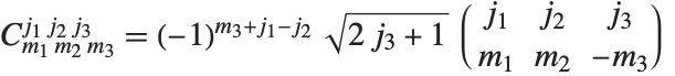 来给出.
来给出.
| Exp[z] | 指数函数 |
| Log[z] | 对数函数 |
| Log[b,z] | 对数函数 |
| Log2[z]
,
Log10[z] | 底数为 2 和 10 的对数函数 |
| Sin[z]
,
Cos[z]
,
Tan[z]
,
Csc[z]
,
Sec[z]
,
Cot[z] | |
三角函数(自变量单位是弧度) | |
| ArcSin[z]
,
ArcCos[z]
,
ArcTan[z]
,
ArcCsc[z]
,
ArcSec[z]
,
ArcCot[z] | |
反三角函数(值为弧度) | |
| ArcTan[x,y] | 自变量为 |
| Sinh[z]
,
Cosh[z]
,
Tanh[z]
,
Csch[z]
,
Sech[z]
,
Coth[z] | |
双曲函数 | |
| ArcSinh[z]
,
ArcCosh[z]
,
ArcTanh[z]
,
ArcCsch[z]
,
ArcSech[z]
,
ArcCoth[z] | |
反双曲函数 | |
| Sinc[z] | sinc 函数 |
| Haversine[z] | 半正矢函数 |
| InverseHaversine[z] | 反半正矢函数 |
| Gudermannian[z] | 古德曼函数 |
| InverseGudermannian[z] | 反古德曼函数 |
通过乘以常数 Degree 可以转化为度:
半正矢函数 Haversine[z] 被定义为  . 反半正矢函数 InverseHaversine[z] 被定义为
  . 古德曼函数 Gudermannian[z] 被定义为
  . 反古德曼函数 InverseGudermannian[z] 被定义为
  . 古德曼函数满足关系如
  . sinc 函数 Sinc[z] 是一个方波信号的傅立叶变换.
求数  的平方根
的平方根  ,实际上就是求方程
  的解. 然而,此方程一般有两个不同的解. 例如,
 和
和  都是方程
都是方程  的解. 但是当用户计算“函数”
  时,通常想得到一个数. 因此必须选择其中一个. 一个标准选择是对
  ,
, 应当是正数. 这正是 Wolfram 语言函数 Sqrt[x] 所做的事情.
有许多数学函数,如求根,本质上给出方程的解. 对数函数和反三角函数是这样的例子. 在几乎所有的情况下,方程有许多可能的解. 但是唯一的“主要”值必须被选择. 这个选择不可能在整个复平面上都是连续的,不连续线或分支线必定出现. 这些分支线的位置常常是相当任意的. Wolfram 语言对它们进行最标准的数学选择.
| Sqrt[z] 和 z^s | |
| Exp[z] | 无 |
| Log[z] | |
三角函数 | 无 |
| ArcSin[z] 和 ArcCos[z] | |
| ArcTan[z] | |
| ArcCsc[z] 和 ArcSec[z] | |
| ArcCot[z] | |
双曲函数 | 无 |
| ArcSinh[z] | |
| ArcCosh[z] | |
| ArcTanh[z] | |
| ArcCsch[z] | |
| ArcSech[z] | |
| ArcCoth[z] |
ArcSin[z] 在分支线两边的值可能是非常不同的:
| I | |
| Infinity | |
| Pi | |
| Degree | |
| GoldenRatio | |
| E | |
| EulerGamma | 欧拉常数 |
| Catalan | Catalan 常数 |
| Khinchin | Khinchin 常数 |
| Glaisher | Glaisher 常数 |
| LegendreP[n,x] | 勒让德多项式 |
| LegendreP[n,m,x] | 相关勒让德多项式 |
| SphericalHarmonicY[l,m,θ,ϕ] | 球面调和函数 |
| GegenbauerC[n,m,x] | 盖根堡多项式 |
| ChebyshevT[n,x]
,
ChebyshevU[n,x] | 第一类和第二类切比雪夫多项式 |
| HermiteH[n,x] | 埃尔米特多项式 |
| LaguerreL[n,x] | 拉盖尔多项式 |
| LaguerreL[n,a,x] | 广义拉盖尔多项式 |
| ZernikeR[n,m,x] | 泽尼克径向多项式 |
| JacobiP[n,a,b,x] | 雅可比多项式 |
切比雪夫多项式级数常常用于函数的数值逼近. 第一类切比雪夫多项式 ChebyshevT[n,x] 由  定义. 它们被规范为
  . 它们满足正交关系:当
  时,
时, .
.  是满足相应于
 的根的
的根的  的离散点处的和式关系.
雅可比多项式 JacobiP[n,a,b,x] 出现在循环群的研究、特别是在量子力学中. 它们满足正交关系:当  时,
时,  . 勒让德、盖根堡、切比雪夫和泽尼克多项式都能看作雅可比多项式的特殊情况. 雅可比多项式有时用另一种形式
  给出.
给出.
可以使用 FindRoot 求特殊函数的根:
在 Wolfram 系统中,特殊函数通常能对自变量的任意复值进行计算. 然而,在本教程中给出的定义关系常常仅适用于自变量的某些特殊选择. 在这些情况下,整个函数相应于这些定义关系的“解析延拓”. 例如,用积分式表达的函数仅当积分存在时才有效,但函数本身通常能通过解析延拓来定义.
伽马函数及相关函数
| Beta[a,b] | 欧拉贝塔函数 |
| Beta[z,a,b] | 不完全贝塔函数 |
| BetaRegularized[z,a,b] | 正则化的不完全贝塔函数 |
| Gamma[z] | 欧拉伽马函数 |
| Gamma[a,z] | 不完全伽马函数 |
| Gamma[a,z0,z1] | 广义不完全伽马函数 |
| GammaRegularized[a,z] | 正则化的不完全伽马函数 |
| InverseBetaRegularized[s,a,b] | 反贝塔函数 |
| InverseGammaRegularized[a,s] | 反伽马函数 |
| Pochhammer[a,n] | Pochhammer 符号 |
| PolyGamma[z] | 双伽玛函数 |
| PolyGamma[n,z] | 双伽玛函数 |
| LogGamma[z] | 欧拉 log-gamma 函数 |
| LogBarnesG[z] | Barnes G 函数的对数 |
| BarnesG[z] | Barnes G 函数 |
| Hyperfactorial[n] | 超阶乘函数 |
在一些运算中,特别是数论中,伽马函数的对数经常出现. 对于正实数自变量,其对数值可以通过 Log[Gamma[z]]. 轻松得到. 然而对于复自变量,该式产生伪不连续性. Wolfram 系统因此另外给出函数 LogGamma[z],它产生具有沿负实轴切割的单个分支线的伽马函数的对数.
Pochhammer 符号或上升阶乘 Pochhammer[a,n] 是  . 它常常出现在超几何函数的级数展开式中. 注意即使当其定义中出现的伽马函数为无穷大时,Pochhammer 符号也有确定的值.
在某些情况下,计算不完全贝塔和伽马函数本身是不方便的,而代之以计算正则化形式,在这个形式中,用完全贝塔和伽马函数除这些函数. Wolfram 系统包含正则化的不完全贝塔函数 BetaRegularized[z,a,b],其定义为  ,且考虑奇点情况. Wolfram 系统还包含正则化的不完全伽马函数 GammaRegularized[a,z],其定义为
  ,且奇点情况被考虑.
不完全贝塔和伽马函数及其反函数在统计学中是常见的. 反贝塔函数 InverseBetaRegularized[s,a,b] 是方程  对
对  的解. 类似地,反伽马函数 InverseGammaRegularized[a,s] 是方程
  对
对  的解.
的解.
伽马函数的导数常出现在有理级数的求和当中. 双伽玛函数 PolyGamma[z] 是伽马函数的对数的导数,由  给出. 对整数自变量,双伽玛函数满足关系
  ,其中
,其中  是欧拉常数 (在 Wolfram 系统中为 EulerGamma),
 是调和数.
是调和数.
多伽马函数 PolyGamma[n,z] 由  给出. 注意双伽玛函数对应于
  . 一般形式
  是
是  阶伽马函数的对数的导数,而非
  阶. 多伽马函数满足关系
  . PolyGamma[ν,z] 由任意复数
  通过分数阶微积分解析延拓得到.
BarnesG[z] 是 Gamma 函数的推广,由泛函恒等式 BarnesG[z+1]=Gamma[z] BarnesG[z] 定义, 其中对于正数 z,BarnesG 的对数的三阶导数是正数. BarnesG 是复平面上的一个整函数.
Zeta 函数及相关函数
| DirichletL[k,j,s] | Dirichlet L-函数 |
| LerchPhi[z,s,a] | Lerch 超越函数 |
| PolyLog[n,z] | 多对数函数 |
| PolyLog[n,p,z] | 尼尔森广义多对数函数 |
| RamanujanTau[n] | Ramanujan |
| RamanujanTauL[n] | Ramanujan |
| RamanujanTauTheta[n] | Ramanujan |
| RamanujanTauZ[n] | Ramanujan |
| RiemannSiegelTheta[t] | 黎曼–西格尔函数 |
| RiemannSiegelZ[t] | 黎曼–西格尔函数 |
| StieltjesGamma[n] | 斯蒂尔吉斯常数 |
| Zeta[s] | 黎曼 ζ 函数 |
| Zeta[s,a] | 广义黎曼 ζ 函数 |
| HurwitzZeta[s,a] | Hurwitz ζ 函数 |
| HurwitzLerchPhi[z,s,a] | Hurwitz–Lerch 超越函数 |
在研究  时,按照
时,按照  和
和  (
( 为实数)定义两个黎曼–西格尔函数 RiemannSiegelZ[t] 和 RiemannSiegelTheta[t] 往往带来方便. 注意黎曼–西格尔函数当
 为实数时,都取实值.
Ramanujan  Dirichlet L-函数 RamanujanTauL[s] 由 L(s)
 (
( ) 定义,其系数为 RamanujanTau[n]. 与黎曼 ζ 函数类似,定义两个函数 RamanujanTauZ[t] 和 RamanujanTauTheta[t] 也会带来方便.
多对数函数 PolyLog[n,z] 由  给出. 多对数函数有时称为 Jonquière 函数. 双对数函数PolyLog[2,z] 满足
  .
.  有时称为 Spence 积分. 尼尔森广义多对数函数或称超对数 PolyLog[n,p,z] 由
  给出. 多对数函数出现在基本粒子物理学或代数 K‐理论的 Feynman 图积分中.
Lerch 超越函数 LerchPhi[z,s,a] 是 ζ 和多对数函数的推广,由  定义,其中
定义,其中  的项被排除. 许多倒数幂的和式能用 Lerch 超越函数来表示. 例如 Catalan 贝塔函数
  可由
可由  来得到.
来得到.
Lerch 超越函数也能用来计算数论中的 Dirichlet L‐级数. 基本的 L‐级数的形式为  ,其中"字符"
  是周期为
是周期为  的整数函数. 这种 L‐级数可以写成 Lerch 函数的和,其中
  是
是  的幂.
的幂.
指数积分及相关函数
| CosIntegral[z] | 余弦积分函数 |
| CoshIntegral[z] | 双曲余弦积分函数 |
| ExpIntegralE[n,z] | 指数积分 En(z) |
| ExpIntegralEi[z] | 指数积分 |
| LogIntegral[z] | 对数积分 |
| SinIntegral[z] | 正弦积分函数 |
| SinhIntegral[z] | 双曲正弦积分函数 |
对数积分函数 LogIntegral[z] 由  (
( )定义,并取积分的主值.
  是数论中系数分布研究的核心. 对数积分函数有时也表示为
  . 在数论的某些应用中,
 被定义为
被定义为  ,且不取主值. 这一定义与 Wolfram 系统中使用的定义相差常数
  .
.
正弦和余弦积分函数 SinIntegral[z] 和 CosIntegral[z] 由  和
和  定义. 双曲正弦和余弦积分函数 SinhIntegral[z] 和 CoshIntegral[z] 由
  和
和  定义.
定义.
误差函数及相关函数
| Erf[z] | 误差函数 |
| Erf[z0,z1] | 广义误差函数 |
| Erfc[z] | 余误差函数 |
| Erfi[z] | 虚数误差函数 |
| FresnelC[z] | 费涅尔积分 C(z) |
| FresnelS[z] | 费涅尔积分 |
| InverseErf[s] | 反误差函数 |
| InverseErfc[s] | 反余误差函数 |
误差函数 Erf[z] 是高斯分布的积分,由  给出. 余误差函数 Erfc[z] 由
 简单地给出. 虚数误差函数 Erfi[z] 由
  给出. 广义误差函数 Erf[z0,z1] 由积分
  定义. 误差函数在统计学的许多计算中是很重要的.
贝塞尔及相关函数
| AiryAi[z] 和 AiryBi[z] | Airy 函数 |
| AiryAiPrime[z] 和 AiryBiPrime[z] | Airy 函数的导数 |
| BesselJ[n,z] 和 BesselY[n,z] | 贝塞尔函数 |
| BesselI[n,z] 和 BesselK[n,z] | 修正贝塞尔函数 |
| KelvinBer[n,z] 和 KelvinBei[n,z] | 开尔文函数 |
| KelvinKer[n,z] 和 KelvinKei[n,z] | 开尔文函数 |
| HankelH1[n,z] 和 HankelH2[n,z] | 汉克尔函数 |
| SphericalBesselJ[n,z] 和 SphericalBesselY[n,z] | |
球贝塞尔函数 | |
| SphericalHankelH1[n,z] 和 SphericalHankelH2[n,z] | |
球汉克尔函数 | |
| StruveH[n,z] 和 StruveL[n,z] | Struve 函数 |
球贝塞尔函数 SphericalBesselJ[n,z] 和 SphericalBesselY[n,z],以及球汉克尔函数 SphericalHankelH1[n,z] 和 SphericalHankelH2[n,z] 出现在球对称波动现象的研究中. 这些函数通过  与普通函数相联系,这里
  和
和  可以是
可以是  和
和  ,
,  和
和  ,或者
,或者  和
和  . 对于整数
  ,使用 FunctionExpand 可以将球面贝塞尔函数展开成普通函数的形式.
特别在电子工程中,人们常常要定义开尔文函数 KelvinBer[n,z], KelvinBei[n,z], KelvinKer[n,z] 和 KelvinKei[n,z]. 这些函数通过  ,
, 与普通贝塞尔函数相联系.
Airy 函数 AiryAi[z] 和 AiryBi[z] 是微分方程  的两个独立解
  和
和  . 当
. 当  趋向于正无穷大时,
 趋向于0,而
  无限增大. Airy 函数与1/3整数阶修正贝塞尔函数相关. Airy 函数常作为边界值问题的解出现在电磁理论和量子力学中. 在许多情况下,也出现 Airy 函数的导数 AiryAiPrime[z] 和 AiryBiPrime[z].
Struve 函数 StruveH[n,z] 出现在对整数  的非齐次贝赛尔方程
  的解中. 这个方程的通解由贝塞尔函数的线性组合加 Struve 函数
  构成. 修正 Struve 函数 StruveL[n,z] 以普通 Struve 函数的形式由
  给出. Struve 函数特别出现在电磁理论中.
| BesselJZero[n,k] | 贝塞尔函数 |
| BesselJZero[n,k,x0] | 大于 |
| BesselYZero[n,k] | 贝塞尔函数 |
| BesselYZero[n,k,x0] | 大于 |
| AiryAiZero[k] | Airy 函数 |
| AiryAiZero[k,x0] | 小于 |
| AiryBiZero[k] | Airy 函数 |
| AiryBiZero[k,x0] | 小于 |
勒让德函数及相关函数
勒让德函数及缔合勒让德函数满足微分方程  . 第一类勒让德函数, LegendreP[n,z] 和 LegendreP[n,m,z],当
  和
和  为整数时,化为勒让德多项式. 第二类勒让德函数LegendreQ[n,z] 和 LegendreQ[n,m,z] 给出微分方程的第二个线性无关解. 对于整数
  ,它们在
,它们在  处有对数奇点.
  和
和  给出微分方程在
  时的解.
时的解.
| LegendreP[n,m,z] 或 LegendreP[n,m,1,z] | |
包含 | |
| LegendreP[n,m,2,z] |
包含 |
| LegendreP[n,m,3,z] | 包含 |
勒让德函数的类型. 对 LegendreQ 存在类似的类型.
用同样的方法,在 GegenbauerC 等等的函数中,指标变量取任意复数就能得到盖根堡函数、切比雪夫函数、厄米函数、雅可比函数和拉盖尔函数. 然而不同于缔合勒让德函数,不需要区分这些函数的不同类型.
超几何函数及其推广
| Hypergeometric0F1[a,z] | 超几何函数 |
| Hypergeometric0F1Regularized[a,z] | 正则化超几何函数 |
| Hypergeometric1F1[a,b,z] | 库默尔合流超几何函数 |
| Hypergeometric1F1Regularized[a,b,z] | 正则化合流超几何函数 |
| HypergeometricU[a,b,z] | 合流超几何函数 |
| WhittakerM[k,m,z] and WhittakerW[k,m,z] | |
惠特克函数 | |
| ParabolicCylinderD[ν,z] | 抛物柱面函数 |
| CoulombF[l,η,ρ] | 规则库伦波函数 |
| CoulombG[l,η,ρ] | 不规则库伦波函数 |
但目前为止,我们所讨论的特殊函数多数都能被看作合流超几何函数 Hypergeometric1F1[a,b,z] 的特殊情形.
惠特克函数 WhittakerM[k,m,z] 和 WhittakerW[k,m,z] 给出正态化的库默尔微分方程(或称为惠特克微分方程)的一对解. 惠特克函数  通过
通过  与
与  相关. 第二个惠特克函数
  服从同一关系,只要由
  代替
代替  .
.
库伦波函数 CoulombF[l,η,ρ] 和 CoulombG[l,η,ρ] 也是合流超几何函数的特殊情形. 库伦波函数给出点核的库伦势中的径向薛定谔方程的解. 正则库伦波函数由  给出,其中
给出,其中  . 不规则 Coulomb 波函数
  由类似的表达式给出,但用
  替换
替换  .
.
| Hypergeometric2F1[a,b,c,z] | 超几何函数 |
| Hypergeometric2F1Regularized[a,b,c,z] | |
正则化的超几何函数 | |
| HypergeometricPFQ[{a1,…,ap},{b1,…,bq},z] | |
广义超几何函数 | |
| HypergeometricPFQRegularized[{a1,…,ap},{b1,…,bq},z] | |
正则化的广义超几何函数 | |
| MeijerG[{{a1,…,an},{an+1,…,ap}},{{b1,…,bm},{bm+1,…,bq}},z] | |
梅杰 G-函数 | |
| AppellF1[a,b1,b2,c,x,y] | 阿佩尔双变量超几何函数 |
梅杰 G-函数 MeijerG[{{a1,…,an},{an+1,…,ap}},{{b1,…,bm},{bm+1,…,bq}},z] 是由围道积分表示式 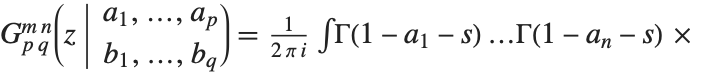
 定义,其中积分的围道设在
  的极点和
的极点和  的极点之间. MeijerG 是一个非常一般的函数,它的特殊情形包括了前几节讨论的大多数函数.
q 级数及相关函数
| QPochhammer[z,q] | |
| QPochhammer[z,q,n] | |
| QFactorial[z,q] | 阶乘的 |
| QBinomial[n,m,q] | 二项式系数的 |
| QGamma[z,q] | 欧拉伽马函数 |
| QPolyGamma[z,q] | |
| QPolyGamma[n,z,q] | |
| QHypergeometricPFQ[{a1,…,ap},{b1,…,bq},q,z] | |
基本超几何级数 | |
有限  Pochhammer 符号
  定义为乘积
定义为乘积  . 其极限
. 其极限  定义了当
定义了当  <1 时的
<1 时的  Pochhammer 符号
  .
.  Pochhammer 符号
  是 Pochhammer
  符号的
符号的  形式. 其在极限

 /(1-q)n 中被复原.
乘积对数函数
| ProductLog[z] | 乘积对数函数 |
球体函数
| SpheroidalS1[n,m,γ,z] 和 SpheroidalS2[n,m,γ,z] | |
径向球体函数 | |
| SpheroidalS1Prime[n,m,γ,z] 和 SpheroidalS2Prime[n,m,γ,z] | |
径向球体函数关于 z 的导数 | |
| SpheroidalPS[n,m,γ,z] 和 SpheroidalQS[n,m,γ,z] | |
角球体函数 | |
| SpheroidalPSPrime[n,m,γ,z] 和 SpheroidalQSPrime[n,m,γ,z] | |
角球体函数关于 z 的导数 | |
| SpheroidalEigenvalue[n,m,γ] | n 阶 m 次的球面特征值 |
径向球体函数 SpheroidalS1[n,m,γ,z] 及 SpheroidalS2[n,m,γ,z] 和角球体函数 SpheroidalPS[n,m,γ,z] 和 SpheroidalQS[n,m,γ,z] 出现在球形区域上波动方程的解中. 这两类函数均为方程  的解. 仅当
  是由 SpheroidalEigenvalue[n,m,γ] 给出的球面特征值时,该方程有可规范化的解. 球体函数也可作为特征函数出现在对傅立叶变换的有限模拟中.
SpheroidalS1 和 SpheroidalS2 是球面贝塞耳函数  和
和  的有效球体对照,而 SpheroidalPS 和SpheroidalQS 则有效对照着勒让德函数
  和
和  .
.  对应着长球面几何,而
  对应着扁球面几何.
■ 振幅 |
■ 自变量 |
■ δ 振幅 |
■ 坐标 |
■ 特征数 |
■ 参数 |
■ 互补参数 |
■ 模 |
■ 模角 |
■ Nome |
■ 不变量 |
■ 半周期 |
■ 周期比 |
■ 判别式 |
■ 曲线 |
■ 坐标 |
| JacobiAmplitude[u,m] | 给出对应于自变量 u 和参数 m 的振幅 ϕ |
| EllipticNomeQ[m] | 给出对应于参数 m 的 nome q |
| InverseEllipticNomeQ[q] | 给出对应于 nome q 的参数 m |
| WeierstrassInvariants[{ω,ω′}] | 给出对应于半周期 {ω,ω′} 的不变量 {g2,g3} |
| WeierstrassHalfPeriods[{g2,g3}] | 给出对应于不变量 {g2,g3} 的半周期 {ω,ω′} |
椭圆积分
| EllipticK[m] | 第一类完全椭圆积分 |
| EllipticF[ϕ,m] | 第一类椭圆积分 |
| EllipticE[m] | 第二类完全椭圆积分 E(m) |
| EllipticE[ϕ,m] | 第二类椭圆积分 E(ϕm) |
| EllipticPi[n,m] | 第三类完全椭圆积分 |
| EllipticPi[n,ϕ,m] | 第三类椭圆积分 |
| JacobiZeta[ϕ,m] | 雅可比 ζ 函数 |
第一类完全椭圆积分 EllipticK[m] 由  给出. 注意
  用来表示第一类完全椭圆积分,而
  用来表示不完全的形式. 在许多应用中,参数
  不是显式给定的,且
  简单记作
简单记作  . 第一类互补完全椭圆积分
  由
由  给出,常被记作
  .
.  和
和  给出"实" 和 "虚" 的相应于 "椭圆函数" 中所讨论的雅可比椭圆函数的四分之一周期.
椭圆函数
| JacobiAmplitude[u,m] | 振幅函数 |
| JacobiSN[u,m]
,
JacobiCN[u,m]
, etc.
| |
雅可比椭圆函数 | |
| InverseJacobiSN[v,m]
,
InverseJacobiCN[v,m]
, etc.
| |
反雅可比椭圆函数 | |
| EllipticTheta[a,u,q] | θ 函数 |
| EllipticThetaPrime[a,u,q] | θ 函数的导数 |
| SiegelTheta[τ,s] | Siegel θ 函数 |
| SiegelTheta[v,τ,s] | Siegel θ 函数 |
| WeierstrassP[u,{g2,g3}] | Weierstrass 椭圆函数 |
| WeierstrassPPrime[u,{g2,g3}] | Weierstrass 椭圆函数的导数 |
| InverseWeierstrassP[p,{g2,g3}] | 反 Weierstrass 椭圆函数 |
| WeierstrassSigma[u,{g2,g3}] | Weierstrass σ 函数 |
| WeierstrassZeta[u,{g2,g3}] | Weierstrass ζ 函数 |
反雅可比椭圆函数 InverseJacobiSN[v,m], InverseJacobiCN[v,m] 等也是 Wolfram 语言的内置函数. 例如反函数  给出
给出  关于
关于  的解. 反雅可比椭圆函数与椭圆积分有关.
EllipticTheta[a,u,q] 中分别取 a 为 1、2、3 和 4 得到四个 θ 函数  . 其定义为
  ,
,  ,
,  ,
,  . θ 函数常写作
  ,其参数
,其参数  常常不写出. θ 函数有时写成
  的形式,其中
  与
与  的关系为
的关系为  . 另外,
. 另外, 有时用
有时用  代替,两者的关系为
  . 所有的 θ 函数满足扩散类微分方程
  .
.
具有向量 s 的 p 维 Riemann 模块方阵(square modular matrix)的 Siegel θ 函数 SiegelTheta[τ,s] 将椭圆 θ 函数推广至复维数 p,其定义为  ,其中 n 跨越(runs over)全部 p 维整数向量. 特征值为 SiegelTheta[ν,τ,s] 的 Siegel θ 函数的定义由
 给出,其中特征数 ν 是一对 p 维向量 {α,β}.
Weierstrass 椭圆函数 WeierstrassP[u,{g2,g3}] 可以被看作是椭圆积分的反函数. Weierstrass 函数 给出
给出  关于
关于  的解. 函数 WeierstrassPPrime[u,{g2,g3}] 由
  给出.
给出.
椭圆模函数
| DedekindEta[τ] | Dedekind η 函数 |
| KleinInvariantJ[τ] | Klein 不变模函数 |
| ModularLambda[τ] | 模 λ 函数 |
广义椭圆积分和函数
| ArithmeticGeometricMean[a,b] | |
| EllipticExp[u,{a,b}] | 与椭圆曲线 |
| EllipticLog[{x,y},{a,b}] | 与椭圆曲线 |
函数 EllipticLog[{x,y},{a,b}] 被定义为积分 的值,其中平方根的正负通过给出使得
  成立的
成立的  值来确定. 形如
  的积分可以用普通对数(和反三角函数)来表示. 可以认为 EllipticLog 给出该积分的推广,其中平方根下的多项式是三次的.
函数 EllipticExp[u,{a,b}] 是 EllipticLog 的反函数. 它返回出现在 EllipticLog 中的列表  . EllipticExp 是一个椭圆函数,在复平面
  上是双周期的.
ArithmeticGeometricMean[a,b] 给出两个数  和
和  的算术-几何平均值(AGM). 该量是计算椭圆积分的和其他函数的许多数值算法的核心. 对于正实数
  和
和  ,其 AGM 按下述方法获得:从
  ,
, 开始,然后重复变换
  ,
, 直到在要求的精度下
  为止.
为止.
| MathieuC[a,q,z] | 具有特征值 a 和参数 q 的 Mathieu 偶函数 |
| MathieuS[b,q,z] | 具有特征值 b 和参数 q 的 Mathieu 奇函数 |
| MathieuCPrime[a,q,z] 和 MathieuSPrime[b,q,z] | Mathieu 函数的 z 导数 |
| MathieuCharacteristicA[r,q] | 具有特征指数 r 和参数 q 的 Mathieu 偶函数的特征值 ar |
| MathieuCharacteristicB[r,q] | 具有特征指数 r 和参数 q 的 Mathieu 奇函数的特征值 br |
| MathieuCharacteristicExponent[a,q] | 具有特征值 a 和参数 q 的 Mathieu 函数的特征指数 r |
Mathieu 函数 MathieuC[a,q,z] 和 MathieuS[a,q,z] 是方程  的解. 这个方程出现在涉及椭圆形状或周期位势的许多物理场合. 函数 MathieuC 定义为关于
  是偶函数,而 MathieuS 是奇函数.
当  时,Mathieu 函数简化为
  和
和  . 对于非零
  ,Mathieu 函数仅对某些
  的值关于
的值关于  是周期的. Mathieu 特征值由 MathieuCharacteristicA[r,q] 和 MathieuCharacteristicB[r,q] 给出,其中
  是整数或有理数. 这些值常记为
  和
和  .
.
根据 Floquet 定理,任何 Mathieu 函数可以用  的形式写出, 其中
  有周期
有周期  ,
,  是 Mathieu 特征指数 MathieuCharacteristicExponent[a,q]. 当特征指数
  是整数或有理数时,Mathieu 函数是周期的. 然而,一般情况下, 当
  不是实整数时,
  和
和  是相等的.
是相等的.
自动计算 | 指定变量的精确结果 |
| N[expr,n] | 任何精度的数值近似 |
| D[expr,x] | 导数的精确结果 |
| N[D[expr,x]] | 导数的数值近似 |
| Series[expr,{x,x0,n}] | 级数展开 |
| Integrate[expr,x] | 积分的精确结果 |
| NIntegrate[expr,x] | 积分的数值近似 |
| FindRoot[expr==0,{x,x0}] | 方程根的数值近似 |
大部分特殊方程有能用基本函数或其他特殊函数表示的导数. 但即使对导数不能明显表示的情况,也能使用 N 求出导数的数值近似值.
使用 N 给出数值近似:
| FullSimplify[expr] | 使用广泛的变换规则化简 expr |
| FunctionExpand[expr] | 展开特殊函数 |
这是的最终结果甚至不涉及 PolyGamma: